What is JupyterLab?¶

interactive python/R programming env
use the computationable power from our HPC
access the HPC data directly

Common usage¶

create a python/R notebook
create table of content and cell tags
[navigation] go to my data dir and start analysis
is my notebook running?
some hotkeys

Data analysis using Pandas¶

read_csv(), head(), sample(), shape(), columns
df.isnull().any().any()
sort_values()
value_counts()
describe()
groupby()
min(),max(),std(),median()
subset dataframe
to_csv()

Example Data: several clinicl measurements of 48 Type 2 diabetes patients and 48 normal individuals¶

[22]:

import pandas as pd
df = pd.read_csv("https://raw.githubusercontent.com/YichaoOU/Data_Science_Tutorials/master/LTC_selected_features.csv",sep=",")

read data¶

[5]:

df.head()

[5]:

	SampleID	Peptide_27	Fasting_plasma_glucose_(mmol/l)	HbA1c	Fasting_plasma_insulin_(pmol/l)	C-Peptide_(nmol/l)	HOMA-IR	Free_fatty_acids_(mmol/l)	Class
0	3	10.42	4.73	6.5	121.4	1.63	3.7	1.03	1
1	5	102.86	7.16	7.6	226.0	1.11	10.4	0.98	1
2	6	9.84	5.06	4.9	39.7	0.75	1.3	0.35	0
3	7	41.03	5.35	6.3	203.3	2.02	7.0	1.17	1
4	8	12.30	5.37	5.6	50.8	1.19	1.7	0.32	0

[6]:

df.sample(n=3)

[6]:

	SampleID	Peptide_27	Fasting_plasma_glucose_(mmol/l)	HbA1c	Fasting_plasma_insulin_(pmol/l)	C-Peptide_(nmol/l)	HOMA-IR	Free_fatty_acids_(mmol/l)	Class
9	13	27.82	5.67	5.8	79.8	1.27	2.9	0.19	0
88	92	11.74	4.90	5.0	135.3	1.04	4.2	0.28	0
60	64	114.61	18.74	10.5	207.0	1.00	24.8	1.16	1

[25]:

df.columns

[25]:

Index(['SampleID', 'Peptide_27', 'Fasting_plasma_glucose_(mmol/l)', 'HbA1c',
       'Fasting_plasma_insulin_(pmol/l)', 'C-Peptide_(nmol/l)', 'HOMA-IR',
       'Free_fatty_acids_(mmol/l)', 'Class'],
      dtype='object')

[7]:

df.isnull().any().any()

[7]:

False

get some statistics from data¶

[8]:

df.describe()

[8]:

	SampleID	Peptide_27	Fasting_plasma_glucose_(mmol/l)	HbA1c	Fasting_plasma_insulin_(pmol/l)	C-Peptide_(nmol/l)	HOMA-IR	Free_fatty_acids_(mmol/l)	Class
count	96.000000	96.000000	96.000000	96.000000	96.000000	96.000000	96.000000	96.000000	96.000000
mean	51.541667	33.570208	6.711146	6.248958	155.566667	1.488632	7.240625	0.630937	0.500000
std	27.961596	23.398125	2.734147	1.455515	141.817693	0.778423	7.617384	0.343940	0.502625
min	3.000000	2.630000	3.800000	4.300000	15.000000	0.310000	0.500000	0.150000	0.000000
25%	27.750000	15.597500	5.037500	5.300000	64.550000	0.935000	2.200000	0.340000	0.000000
50%	51.500000	27.280000	5.670000	5.750000	112.600000	1.235000	4.100000	0.550000	0.500000
75%	75.250000	46.885000	7.352500	6.625000	199.775000	1.845000	10.125000	0.940000	1.000000
max	100.000000	114.610000	18.740000	10.900000	783.000000	4.180000	45.300000	1.350000	1.000000

[9]:

df = df.sort_values("HbA1c",ascending=False)

[10]:

df.head()

[10]:

	SampleID	Peptide_27	Fasting_plasma_glucose_(mmol/l)	HbA1c	Fasting_plasma_insulin_(pmol/l)	C-Peptide_(nmol/l)	HOMA-IR	Free_fatty_acids_(mmol/l)	Class
55	59	55.81	9.71	10.9	212.0	2.26	13.2	0.39	1
19	23	53.11	8.24	10.8	242.0	2.42	12.8	0.83	1
62	66	23.47	10.13	10.7	143.1	1.02	9.3	0.92	1
60	64	114.61	18.74	10.5	207.0	1.00	24.8	1.16	1
85	89	56.46	9.89	9.1	178.2	0.94	11.3	1.17	1

[12]:

df.value_counts('Class')

[12]:

Class
0    48
1    48
dtype: int64

[13]:

df.shape

[13]:

(96, 9)

[14]:

df['HbA1c'].min()

[14]:

4.3

[15]:

df['HbA1c'].median()

[15]:

5.75

[42]:

df['HbA1c'].max()

[42]:

10.9

[16]:

df.groupby('Class').mean()

[16]:

	SampleID	Peptide_27	Fasting_plasma_glucose_(mmol/l)	HbA1c	Fasting_plasma_insulin_(pmol/l)	C-Peptide_(nmol/l)	HOMA-IR	Free_fatty_acids_(mmol/l)
Class
0	53.354167	21.965417	5.321667	5.345833	79.208333	1.103513	2.679167	0.391042
1	49.729167	45.175000	8.100625	7.152083	231.925000	1.873750	11.802083	0.870833

[21]:

df.groupby('Class').head()

[21]:

	SampleID	Peptide_27	Fasting_plasma_glucose_(mmol/l)	HbA1c	Fasting_plasma_insulin_(pmol/l)	C-Peptide_(nmol/l)	HOMA-IR	Free_fatty_acids_(mmol/l)	Class
55	59	55.81	9.71	10.9	212.0	2.26	13.2	0.39	1
19	23	53.11	8.24	10.8	242.0	2.42	12.8	0.83	1
62	66	23.47	10.13	10.7	143.1	1.02	9.3	0.92	1
60	64	114.61	18.74	10.5	207.0	1.00	24.8	1.16	1
85	89	56.46	9.89	9.1	178.2	0.94	11.3	1.17	1
89	93	18.06	7.39	6.5	88.9	1.22	4.2	0.35	0
65	69	43.86	6.26	6.0	69.2	1.20	2.8	0.22	0
43	47	11.36	6.67	5.9	58.2	0.89	2.5	0.36	0
35	39	32.81	5.68	5.9	102.4	1.03	3.7	0.27	0
6	10	25.75	5.67	5.8	67.1	0.94	2.4	0.26	0

[41]:

df.groupby('Class').head().to_csv("My_examlpe.tsv",index=False,sep="\t")

subset data¶

[60]:

df_undiagnosed = df[df['HbA1c']<6.5]

[61]:

df_undiagnosed['Class'].value_counts()

[61]:

0    47
1    18
Name: Class, dtype: int64

[62]:

df_undiagnosed['Class'].value_counts(normalize=True)

[62]:

0    0.723077
1    0.276923
Name: Class, dtype: float64

[26]:

data2 = "https://raw.githubusercontent.com/YichaoOU/Data_Science_Tutorials/master/newly_diagnosed.csv"

Exercise¶

Read this table as Pandas object¶

[36]:

df2 = pd.read_csv(data2,sep=",")

[38]:

df2.head()

[38]:

	Sample ID	Peptide 1	Peptide 2	Peptide 3	Peptide 4	Peptide 5	Peptide 6	Peptide 7	Peptide 8	Peptide 9	...	TSH (mU/l)	fT3 (pmol/l)	fT4 (pmol/l)	Cortisol (nmol/l)	Testosteron (nmol/l)	HOMA-IR	Free fatty acids (mmol/l)	RRsys (mmHg)	RR dia (mmHg)	ssCRP (mg/dl)
0	sample 2	33.58	7.18	9.35	3.57	94.44	14.91	153.05	35.52	9.76	...	0.72	5.23	21.5	NaN	NaN	7.2	0.30	NaN	NaN	0.48
1	sample 3	37.57	8.70	10.79	3.36	94.11	15.99	198.88	39.65	8.62	...	0.97	NaN	NaN	NaN	NaN	9.3	1.04	NaN	NaN	7.15
2	sample 4	27.31	5.42	5.64	2.75	67.01	11.91	148.32	28.90	5.64	...	1.02	5.01	17.6	NaN	NaN	9.1	0.37	NaN	NaN	NaN
3	sample 5	29.09	5.81	4.69	3.61	65.99	12.42	154.55	26.48	6.38	...	1.00	4.61	15.7	NaN	NaN	24.5	0.99	168.0	95.0	0.20
4	sample 6	41.13	8.40	8.85	3.56	109.13	17.60	209.62	44.35	10.43	...	1.30	5.43	19.2	NaN	NaN	11.1	0.54	165.0	84.0	0.30

5 rows × 69 columns

What are the features (columns) in this dataset?¶

[40]:

df2.columns

[40]:

Index(['Sample ID', 'Peptide 1', 'Peptide 2', 'Peptide 3', 'Peptide 4',
       'Peptide 5', 'Peptide 6', 'Peptide 7', 'Peptide 8', 'Peptide 9',
       'Peptide 10', 'Peptide 11', 'Peptide 12', 'Peptide 13', 'Peptide 14',
       'Peptide 15', 'Peptide 16', 'Peptide 17', 'Peptide 18', 'Peptide 21',
       'Peptide 22', 'Peptide 23', 'Peptide 24', 'Peptide 25', 'Peptide 26',
       'Peptide 27', 'Peptide 29', 'Peptide 30', 'Age', 'Diagnosis', 'BMI',
       'HbA1c (%)', 'Gender', 'Height', 'Body weight', 'BMI.1', 'Body fat',
       'Fat free mass', 'Waist', 'Hip', 'WHR', 'Hemoglobin', 'Erythrozyten',
       'Thrombozyten', 'Leukocytes', 'ALAT', 'ASAT', 'gGT',
       'Fasting plasma glucose (mmol/l)', 'Fasting plasma insulin (pmol/l)',
       'C-Peptide (nmol/l)', 'Proinsulin (pmol/l)', 'Creatinin',
       'Triglycerides (mmol/l)', 'Cholesterol total (mmol/l)',
       'HDL-Cholesterol (mmol/l)', 'LDL-Cholesterol (mmol/l)',
       'Proteins total (g/l)', 'Albumin (g/l)', 'TSH (mU/l)', 'fT3 (pmol/l)',
       'fT4 (pmol/l)', 'Cortisol (nmol/l)', 'Testosteron (nmol/l)', 'HOMA-IR',
       'Free fatty acids (mmol/l)', 'RRsys (mmHg)', 'RR dia (mmHg)',
       'ssCRP (mg/dl)'],
      dtype='object')

What are the maximum and minimum values for HbA1c? Are they the same as the first dataset?¶

[45]:

df2['HbA1c (%)'].min()

[45]:

4.3

[46]:

df2['HbA1c (%)'].max()

[46]:

9.7

Does our data have NaN values?¶

[47]:

df2.isnull().any().any()

[47]:

True

[52]:

df2[df2.isnull().any(axis=1)] # any rows containing NaN

[52]:

	Sample ID	Peptide 1	Peptide 2	Peptide 3	Peptide 4	Peptide 5	Peptide 6	Peptide 7	Peptide 8	Peptide 9	...	TSH (mU/l)	fT3 (pmol/l)	fT4 (pmol/l)	Cortisol (nmol/l)	Testosteron (nmol/l)	HOMA-IR	Free fatty acids (mmol/l)	RRsys (mmHg)	RR dia (mmHg)	ssCRP (mg/dl)
0	sample 2	33.58	7.18	9.35	3.57	94.44	14.91	153.05	35.52	9.76	...	0.72	5.23	21.5	NaN	NaN	7.2	0.30	NaN	NaN	0.48
1	sample 3	37.57	8.70	10.79	3.36	94.11	15.99	198.88	39.65	8.62	...	0.97	NaN	NaN	NaN	NaN	9.3	1.04	NaN	NaN	7.15
2	sample 4	27.31	5.42	5.64	2.75	67.01	11.91	148.32	28.90	5.64	...	1.02	5.01	17.6	NaN	NaN	9.1	0.37	NaN	NaN	NaN
3	sample 5	29.09	5.81	4.69	3.61	65.99	12.42	154.55	26.48	6.38	...	1.00	4.61	15.7	NaN	NaN	24.5	0.99	168.0	95.0	0.20
4	sample 6	41.13	8.40	8.85	3.56	109.13	17.60	209.62	44.35	10.43	...	1.30	5.43	19.2	NaN	NaN	11.1	0.54	165.0	84.0	0.30
...	...	...	...	...	...	...	...	...	...	...	...	...	...	...	...	...	...	...	...	...	...
91	Sample 96	26.08	3.54	0.68	0.05	29.46	9.27	142.70	18.61	2.49	...	3.84	NaN	NaN	20.30	117.00	0.8	0.44	130.0	80.0	5.50
92	Sample 97	17.72	2.28	0.64	0.01	19.22	7.37	102.24	13.22	1.61	...	0.63	NaN	NaN	9.73	208.00	5.0	0.36	NaN	NaN	NaN
93	Sample 98	17.70	2.23	0.59	0.01	18.47	5.80	103.94	13.67	1.65	...	1.36	NaN	NaN	9.03	56.00	2.7	0.39	NaN	NaN	NaN
94	Sample 99	26.57	3.33	0.71	0.07	27.69	8.31	137.81	20.68	2.99	...	0.71	NaN	NaN	NaN	1.49	4.6	0.76	NaN	NaN	0.08
95	Sample 100	25.26	3.40	0.64	0.05	27.47	8.72	138.50	19.72	2.54	...	3.34	NaN	NaN	11.50	93.00	4.7	0.35	NaN	NaN	19.50

96 rows × 69 columns

[56]:

df2[df2.columns[df2.isnull().any(axis=0)]] # any columns containing NaN

[56]:

	Body fat	Fat free mass	Waist	Hip	WHR	Hemoglobin	Erythrozyten	Thrombozyten	Leukocytes	ALAT	...	Proteins total (g/l)	Albumin (g/l)	TSH (mU/l)	fT3 (pmol/l)	fT4 (pmol/l)	Cortisol (nmol/l)	Testosteron (nmol/l)	RRsys (mmHg)	RR dia (mmHg)	ssCRP (mg/dl)
0	32.7	73.4	NaN	NaN	NaN	8.3	4.32	216.0	7.4	0.29	...	70.8	NaN	0.72	5.23	21.5	NaN	NaN	NaN	NaN	0.48
1	33.9	NaN	NaN	NaN	NaN	8.9	5.44	180.0	5.9	1.40	...	NaN	NaN	0.97	NaN	NaN	NaN	NaN	NaN	NaN	7.15
2	33.8	NaN	NaN	NaN	NaN	8.9	4.68	169.0	5.4	0.55	...	66.1	NaN	1.02	5.01	17.6	NaN	NaN	NaN	NaN	NaN
3	NaN	NaN	NaN	NaN	NaN	8.5	4.83	237.0	6.6	0.57	...	72.1	NaN	1.00	4.61	15.7	NaN	NaN	168.0	95.0	0.20
4	NaN	NaN	NaN	NaN	NaN	NaN	NaN	NaN	NaN	0.65	...	76.3	NaN	1.30	5.43	19.2	NaN	NaN	165.0	84.0	0.30
...	...	...	...	...	...	...	...	...	...	...	...	...	...	...	...	...	...	...	...	...	...
91	28.0	73.6	NaN	NaN	NaN	10.1	5.28	170.0	8.5	0.65	...	67.9	43.6	3.84	NaN	NaN	20.30	117.00	130.0	80.0	5.50
92	37.9	81.2	NaN	NaN	NaN	7.4	4.18	395.0	10.1	0.30	...	NaN	NaN	0.63	NaN	NaN	9.73	208.00	NaN	NaN	NaN
93	36.8	79.5	NaN	NaN	NaN	9.1	4.76	172.0	7.8	0.43	...	NaN	NaN	1.36	NaN	NaN	9.03	56.00	NaN	NaN	NaN
94	46.9	66.7	135.0	137.0	0.99	8.3	4.84	196.0	5.9	0.43	...	NaN	NaN	0.71	NaN	NaN	NaN	1.49	NaN	NaN	0.08
95	30.6	90.4	NaN	NaN	NaN	8.5	4.61	219.0	3.7	1.16	...	NaN	NaN	3.34	NaN	NaN	11.50	93.00	NaN	NaN	19.50

96 rows × 28 columns

How many diabetic patents will be undiagnosed using HbA1c < 6.5?¶

[64]:

df2_undiagnosed = df2[df2['HbA1c (%)']<6.5]

[67]:

df2_undiagnosed['Diagnosis'].value_counts()

[67]:

NGT    48
T2D    23
Name: Diagnosis, dtype: int64

[68]:

df2_undiagnosed['Diagnosis'].value_counts(normalize=True)

[68]:

NGT    0.676056
T2D    0.323944
Name: Diagnosis, dtype: float64

Save the undiagnosed table as “happy_learning.csv”¶

Data visualization using Seaborn and many other libraries¶

scatter plot
barplot
boxplot
violin plot
beeswarm plot

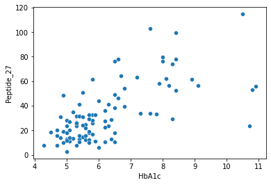
Scatter plots¶

[69]:

import seaborn as sns

[71]:

df.columns

[71]:

Index(['SampleID', 'Peptide_27', 'Fasting_plasma_glucose_(mmol/l)', 'HbA1c',
       'Fasting_plasma_insulin_(pmol/l)', 'C-Peptide_(nmol/l)', 'HOMA-IR',
       'Free_fatty_acids_(mmol/l)', 'Class'],
      dtype='object')

[72]:

sns.scatterplot(data = df,x="HbA1c",y="Peptide_27")

[72]:

<AxesSubplot:xlabel='HbA1c', ylabel='Peptide_27'>

../../_images/content_Bioinformatics_Core_Competencies_Introduction_6_21_2021_v2_53_1.png

[73]:

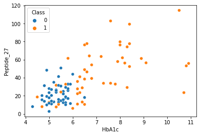
sns.scatterplot(data = df,x="HbA1c",y="Peptide_27",hue="Class")

[73]:

<AxesSubplot:xlabel='HbA1c', ylabel='Peptide_27'>

../../_images/content_Bioinformatics_Core_Competencies_Introduction_6_21_2021_v2_54_1.png

[74]:

import matplotlib.pylab as plt

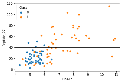
[76]:

sns.scatterplot(data = df,x="HbA1c",y="Peptide_27",hue="Class")
plt.axhline(40,color="black")

[76]:

<matplotlib.lines.Line2D at 0x2aad6a85d6d0>

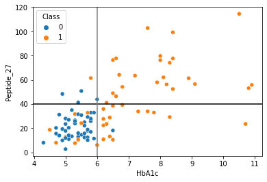
../../_images/content_Bioinformatics_Core_Competencies_Introduction_6_21_2021_v2_56_1.png

[78]:

sns.scatterplot(data = df,x="HbA1c",y="Peptide_27",hue="Class")
plt.axhline(40,color="black")
plt.axvline(6,color="grey")

[78]:

<matplotlib.lines.Line2D at 0x2aad6aa23130>

../../_images/content_Bioinformatics_Core_Competencies_Introduction_6_21_2021_v2_57_1.png

[124]:

import plotly.express as px
import plotly.io as pio
pio.renderers.default = "iframe"

[140]:

df.head()

[140]:

	SampleID	Peptide_27	Fasting_plasma_glucose_(mmol/l)	HbA1c	Fasting_plasma_insulin_(pmol/l)	C-Peptide_(nmol/l)	HOMA-IR	Free_fatty_acids_(mmol/l)	Class
0	3	10.42	4.73	6.5	121.4	1.63	3.7	1.03	1
1	5	102.86	7.16	7.6	226.0	1.11	10.4	0.98	1
2	6	9.84	5.06	4.9	39.7	0.75	1.3	0.35	0
3	7	41.03	5.35	6.3	203.3	2.02	7.0	1.17	1
4	8	12.30	5.37	5.6	50.8	1.19	1.7	0.32	0

interactive scatter plot¶

[142]:

px.scatter(data_frame = df,x="HbA1c",y="Peptide_27",color="Class",hover_data=["SampleID"])

[79]:

df.describe()

[79]:

	SampleID	Peptide_27	Fasting_plasma_glucose_(mmol/l)	HbA1c	Fasting_plasma_insulin_(pmol/l)	C-Peptide_(nmol/l)	HOMA-IR	Free_fatty_acids_(mmol/l)	Class
count	96.000000	96.000000	96.000000	96.000000	96.000000	96.000000	96.000000	96.000000	96.000000
mean	51.541667	33.570208	6.711146	6.248958	155.566667	1.488632	7.240625	0.630937	0.500000
std	27.961596	23.398125	2.734147	1.455515	141.817693	0.778423	7.617384	0.343940	0.502625
min	3.000000	2.630000	3.800000	4.300000	15.000000	0.310000	0.500000	0.150000	0.000000
25%	27.750000	15.597500	5.037500	5.300000	64.550000	0.935000	2.200000	0.340000	0.000000
50%	51.500000	27.280000	5.670000	5.750000	112.600000	1.235000	4.100000	0.550000	0.500000
75%	75.250000	46.885000	7.352500	6.625000	199.775000	1.845000	10.125000	0.940000	1.000000
max	100.000000	114.610000	18.740000	10.900000	783.000000	4.180000	45.300000	1.350000	1.000000

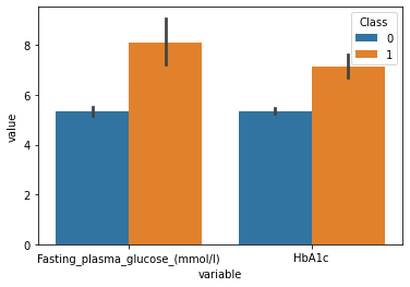
barplot¶

[83]:

plot_df = df.melt(id_vars=['Class'],value_vars = ['Fasting_plasma_glucose_(mmol/l)','HbA1c'])
sns.barplot(data=plot_df,x="variable",y="value",hue="Class")

[83]:

<AxesSubplot:xlabel='variable', ylabel='value'>

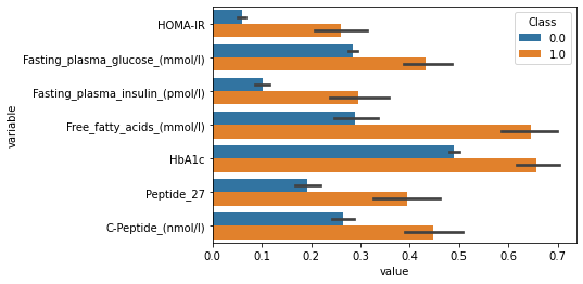
../../_images/content_Bioinformatics_Core_Competencies_Introduction_6_21_2021_v2_64_1.png

[166]:

df_norm = df/df.max(axis=0)
df_norm.head()

[166]:

	SampleID	Peptide_27	Fasting_plasma_glucose_(mmol/l)	HbA1c	Fasting_plasma_insulin_(pmol/l)	C-Peptide_(nmol/l)	HOMA-IR	Free_fatty_acids_(mmol/l)	Class
0	0.03	0.090917	0.252401	0.596330	0.155045	0.389952	0.081678	0.762963	1.0
1	0.05	0.897478	0.382070	0.697248	0.288633	0.265550	0.229581	0.725926	1.0
2	0.06	0.085856	0.270011	0.449541	0.050702	0.179426	0.028698	0.259259	0.0
3	0.07	0.357997	0.285486	0.577982	0.259642	0.483254	0.154525	0.866667	1.0
4	0.08	0.107320	0.286553	0.513761	0.064879	0.284689	0.037528	0.237037	0.0

[175]:

plot_df = df_norm.melt(id_vars=['Class'],value_vars =list(set(df_norm.columns)-set(['Class','SampleID'])) )
sns.barplot(data=plot_df,y="variable",x="value",hue="Class")

[175]:

<AxesSubplot:xlabel='value', ylabel='variable'>

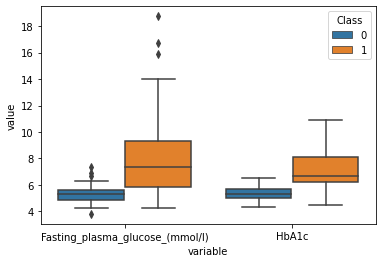
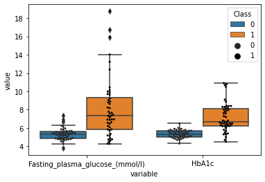
../../_images/content_Bioinformatics_Core_Competencies_Introduction_6_21_2021_v2_66_1.png

boxplot¶

[84]:

sns.boxplot(data=plot_df,x="variable",y="value",hue="Class")

[84]:

<AxesSubplot:xlabel='variable', ylabel='value'>

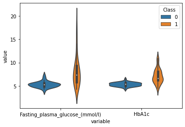
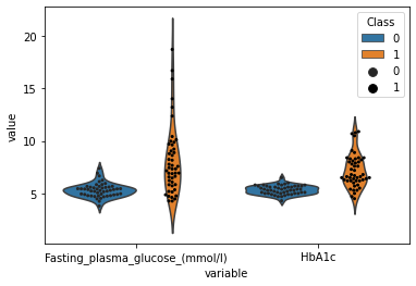
../../_images/content_Bioinformatics_Core_Competencies_Introduction_6_21_2021_v2_68_1.png

Violinplot¶

[86]:

sns.violinplot(data=plot_df,x="variable",y="value",hue="Class")

[86]:

<AxesSubplot:xlabel='variable', ylabel='value'>

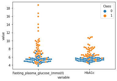
../../_images/content_Bioinformatics_Core_Competencies_Introduction_6_21_2021_v2_70_1.png

beeswarm plot¶

[89]:

sns.swarmplot(data=plot_df,x="variable",y="value",hue="Class")

[89]:

<AxesSubplot:xlabel='variable', ylabel='value'>

../../_images/content_Bioinformatics_Core_Competencies_Introduction_6_21_2021_v2_72_1.png

[100]:

sns.violinplot(data=plot_df,x="variable",y="value",hue="Class",inner=None)
sns.swarmplot(data=plot_df,x="variable",y="value",hue="Class",dodge=True,color="black",s=3)

[100]:

<AxesSubplot:xlabel='variable', ylabel='value'>

../../_images/content_Bioinformatics_Core_Competencies_Introduction_6_21_2021_v2_73_1.png

[101]:

sns.boxplot(data=plot_df,x="variable",y="value",hue="Class")
sns.swarmplot(data=plot_df,x="variable",y="value",hue="Class",dodge=True,color="black",s=3)

[101]:

<AxesSubplot:xlabel='variable', ylabel='value'>

../../_images/content_Bioinformatics_Core_Competencies_Introduction_6_21_2021_v2_74_1.png

[102]:

df.head()

[102]:

	SampleID	Peptide_27	Fasting_plasma_glucose_(mmol/l)	HbA1c	Fasting_plasma_insulin_(pmol/l)	C-Peptide_(nmol/l)	HOMA-IR	Free_fatty_acids_(mmol/l)	Class
0	3	10.42	4.73	6.5	121.4	1.63	3.7	1.03	1
1	5	102.86	7.16	7.6	226.0	1.11	10.4	0.98	1
2	6	9.84	5.06	4.9	39.7	0.75	1.3	0.35	0
3	7	41.03	5.35	6.3	203.3	2.02	7.0	1.17	1
4	8	12.30	5.37	5.6	50.8	1.19	1.7	0.32	0

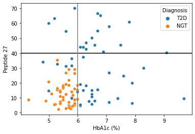
Exercise¶

Can we still use the same HbA1c and Peptide27 cutoff for the second data?¶

[160]:

df2.columns

[160]:

Index(['Sample ID', 'Peptide 1', 'Peptide 2', 'Peptide 3', 'Peptide 4',
       'Peptide 5', 'Peptide 6', 'Peptide 7', 'Peptide 8', 'Peptide 9',
       'Peptide 10', 'Peptide 11', 'Peptide 12', 'Peptide 13', 'Peptide 14',
       'Peptide 15', 'Peptide 16', 'Peptide 17', 'Peptide 18', 'Peptide 21',
       'Peptide 22', 'Peptide 23', 'Peptide 24', 'Peptide 25', 'Peptide 26',
       'Peptide 27', 'Peptide 29', 'Peptide 30', 'Age', 'Diagnosis', 'BMI',
       'HbA1c (%)', 'Gender', 'Height', 'Body weight', 'BMI.1', 'Body fat',
       'Fat free mass', 'Waist', 'Hip', 'WHR', 'Hemoglobin', 'Erythrozyten',
       'Thrombozyten', 'Leukocytes', 'ALAT', 'ASAT', 'gGT',
       'Fasting plasma glucose (mmol/l)', 'Fasting plasma insulin (pmol/l)',
       'C-Peptide (nmol/l)', 'Proinsulin (pmol/l)', 'Creatinin',
       'Triglycerides (mmol/l)', 'Cholesterol total (mmol/l)',
       'HDL-Cholesterol (mmol/l)', 'LDL-Cholesterol (mmol/l)',
       'Proteins total (g/l)', 'Albumin (g/l)', 'TSH (mU/l)', 'fT3 (pmol/l)',
       'fT4 (pmol/l)', 'Cortisol (nmol/l)', 'Testosteron (nmol/l)', 'HOMA-IR',
       'Free fatty acids (mmol/l)', 'RRsys (mmHg)', 'RR dia (mmHg)',
       'ssCRP (mg/dl)'],
      dtype='object')

[161]:

sns.scatterplot(data = df2,x="HbA1c (%)",y="Peptide 27",hue="Diagnosis")
plt.axhline(40,color="black")
plt.axvline(6,color="grey")

[161]:

<matplotlib.lines.Line2D at 0x2aab879ffd90>

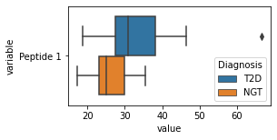
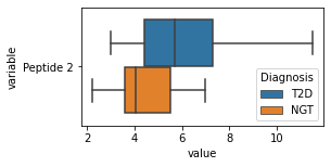
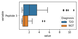
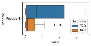
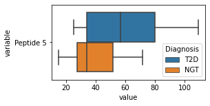
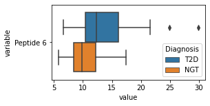
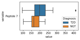
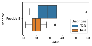
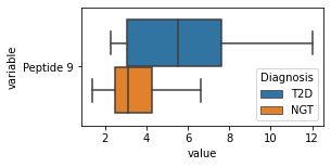
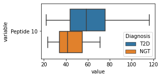
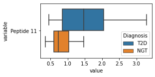
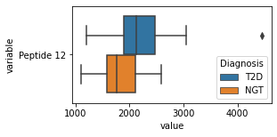
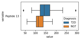
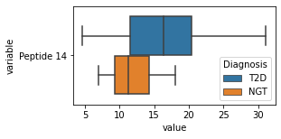
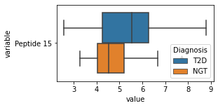
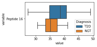
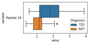
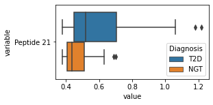
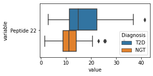
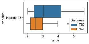
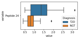
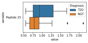
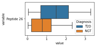
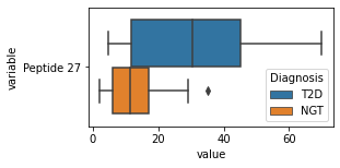
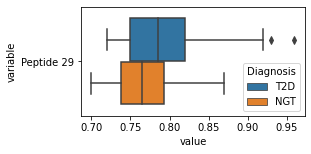
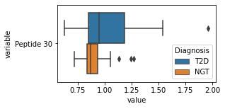
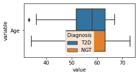
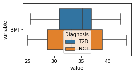
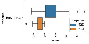
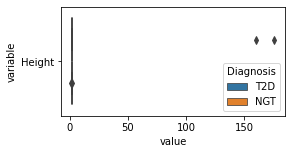
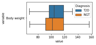
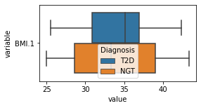
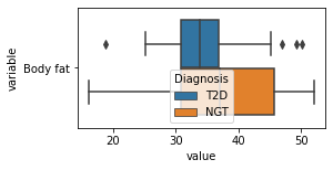
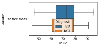
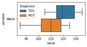
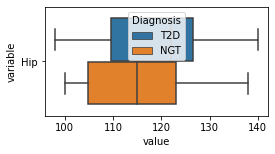
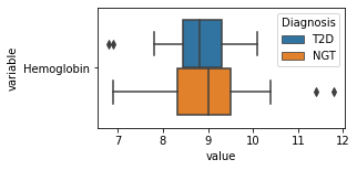
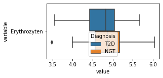
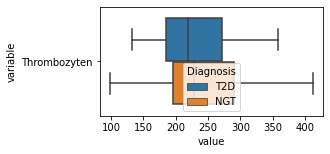
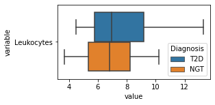
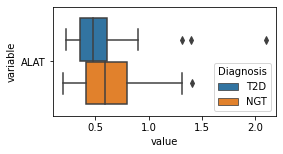
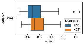
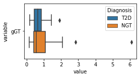
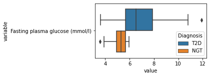
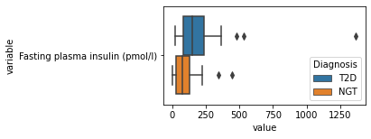
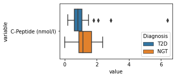
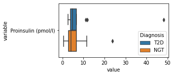
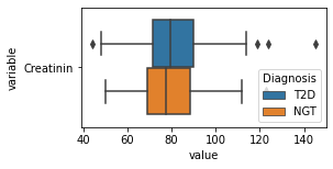
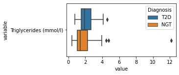
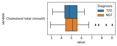
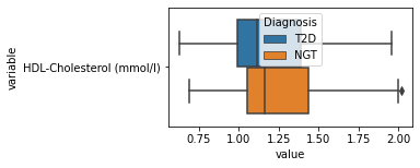
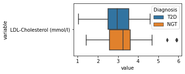
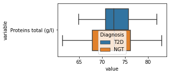
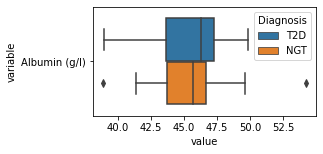
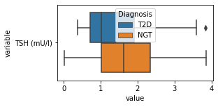
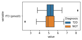
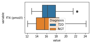
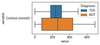
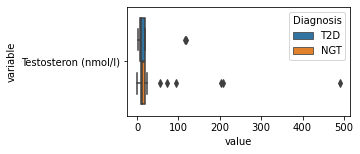
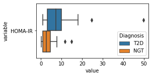
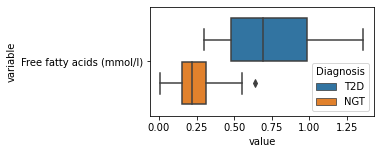
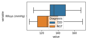
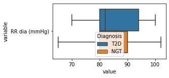
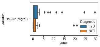
../../_images/content_Bioinformatics_Core_Competencies_Introduction_6_21_2021_v2_79_1.png

what is the data distribution for each feature?¶

[179]:

df2.head()

[179]:

	Sample ID	Peptide 1	Peptide 2	Peptide 3	Peptide 4	Peptide 5	Peptide 6	Peptide 7	Peptide 8	Peptide 9	...	TSH (mU/l)	fT3 (pmol/l)	fT4 (pmol/l)	Cortisol (nmol/l)	Testosteron (nmol/l)	HOMA-IR	Free fatty acids (mmol/l)	RRsys (mmHg)	RR dia (mmHg)	ssCRP (mg/dl)
0	sample 2	33.58	7.18	9.35	3.57	94.44	14.91	153.05	35.52	9.76	...	0.72	5.23	21.5	NaN	NaN	7.2	0.30	NaN	NaN	0.48
1	sample 3	37.57	8.70	10.79	3.36	94.11	15.99	198.88	39.65	8.62	...	0.97	NaN	NaN	NaN	NaN	9.3	1.04	NaN	NaN	7.15
2	sample 4	27.31	5.42	5.64	2.75	67.01	11.91	148.32	28.90	5.64	...	1.02	5.01	17.6	NaN	NaN	9.1	0.37	NaN	NaN	NaN
3	sample 5	29.09	5.81	4.69	3.61	65.99	12.42	154.55	26.48	6.38	...	1.00	4.61	15.7	NaN	NaN	24.5	0.99	168.0	95.0	0.20
4	sample 6	41.13	8.40	8.85	3.56	109.13	17.60	209.62	44.35	10.43	...	1.30	5.43	19.2	NaN	NaN	11.1	0.54	165.0	84.0	0.30

5 rows × 69 columns

[200]:

for c in df2.columns:
    try:
        plt.figure(figsize=(4,2))
        tmp = df2.melt(id_vars=['Diagnosis'],value_vars=c)
        sns.boxplot(data=tmp,y="variable",x="value",hue="Diagnosis")
    except:
        continue

<ipython-input-200-795c994e6a81>:3: RuntimeWarning:

More than 20 figures have been opened. Figures created through the pyplot interface (`matplotlib.pyplot.figure`) are retained until explicitly closed and may consume too much memory. (To control this warning, see the rcParam `figure.max_open_warning`).

<Figure size 288x144 with 0 Axes>

../../_images/content_Bioinformatics_Core_Competencies_Introduction_6_21_2021_v2_82_2.png

../../_images/content_Bioinformatics_Core_Competencies_Introduction_6_21_2021_v2_82_3.png

../../_images/content_Bioinformatics_Core_Competencies_Introduction_6_21_2021_v2_82_4.png

../../_images/content_Bioinformatics_Core_Competencies_Introduction_6_21_2021_v2_82_5.png

../../_images/content_Bioinformatics_Core_Competencies_Introduction_6_21_2021_v2_82_6.png

../../_images/content_Bioinformatics_Core_Competencies_Introduction_6_21_2021_v2_82_7.png

../../_images/content_Bioinformatics_Core_Competencies_Introduction_6_21_2021_v2_82_8.png

../../_images/content_Bioinformatics_Core_Competencies_Introduction_6_21_2021_v2_82_9.png

../../_images/content_Bioinformatics_Core_Competencies_Introduction_6_21_2021_v2_82_10.png

../../_images/content_Bioinformatics_Core_Competencies_Introduction_6_21_2021_v2_82_11.png

../../_images/content_Bioinformatics_Core_Competencies_Introduction_6_21_2021_v2_82_12.png

../../_images/content_Bioinformatics_Core_Competencies_Introduction_6_21_2021_v2_82_13.png

../../_images/content_Bioinformatics_Core_Competencies_Introduction_6_21_2021_v2_82_14.png

../../_images/content_Bioinformatics_Core_Competencies_Introduction_6_21_2021_v2_82_15.png

../../_images/content_Bioinformatics_Core_Competencies_Introduction_6_21_2021_v2_82_16.png

../../_images/content_Bioinformatics_Core_Competencies_Introduction_6_21_2021_v2_82_17.png

../../_images/content_Bioinformatics_Core_Competencies_Introduction_6_21_2021_v2_82_18.png

../../_images/content_Bioinformatics_Core_Competencies_Introduction_6_21_2021_v2_82_19.png

../../_images/content_Bioinformatics_Core_Competencies_Introduction_6_21_2021_v2_82_20.png

../../_images/content_Bioinformatics_Core_Competencies_Introduction_6_21_2021_v2_82_21.png

../../_images/content_Bioinformatics_Core_Competencies_Introduction_6_21_2021_v2_82_22.png

../../_images/content_Bioinformatics_Core_Competencies_Introduction_6_21_2021_v2_82_23.png

../../_images/content_Bioinformatics_Core_Competencies_Introduction_6_21_2021_v2_82_24.png

../../_images/content_Bioinformatics_Core_Competencies_Introduction_6_21_2021_v2_82_25.png

../../_images/content_Bioinformatics_Core_Competencies_Introduction_6_21_2021_v2_82_26.png

../../_images/content_Bioinformatics_Core_Competencies_Introduction_6_21_2021_v2_82_27.png

../../_images/content_Bioinformatics_Core_Competencies_Introduction_6_21_2021_v2_82_28.png

../../_images/content_Bioinformatics_Core_Competencies_Introduction_6_21_2021_v2_82_29.png

<Figure size 288x144 with 0 Axes>

../../_images/content_Bioinformatics_Core_Competencies_Introduction_6_21_2021_v2_82_31.png

../../_images/content_Bioinformatics_Core_Competencies_Introduction_6_21_2021_v2_82_32.png

<Figure size 288x144 with 0 Axes>

../../_images/content_Bioinformatics_Core_Competencies_Introduction_6_21_2021_v2_82_34.png

../../_images/content_Bioinformatics_Core_Competencies_Introduction_6_21_2021_v2_82_35.png

../../_images/content_Bioinformatics_Core_Competencies_Introduction_6_21_2021_v2_82_36.png

../../_images/content_Bioinformatics_Core_Competencies_Introduction_6_21_2021_v2_82_37.png

../../_images/content_Bioinformatics_Core_Competencies_Introduction_6_21_2021_v2_82_38.png

../../_images/content_Bioinformatics_Core_Competencies_Introduction_6_21_2021_v2_82_39.png

../../_images/content_Bioinformatics_Core_Competencies_Introduction_6_21_2021_v2_82_40.png

<Figure size 288x144 with 0 Axes>

../../_images/content_Bioinformatics_Core_Competencies_Introduction_6_21_2021_v2_82_42.png

../../_images/content_Bioinformatics_Core_Competencies_Introduction_6_21_2021_v2_82_43.png

../../_images/content_Bioinformatics_Core_Competencies_Introduction_6_21_2021_v2_82_44.png

../../_images/content_Bioinformatics_Core_Competencies_Introduction_6_21_2021_v2_82_45.png

../../_images/content_Bioinformatics_Core_Competencies_Introduction_6_21_2021_v2_82_46.png

../../_images/content_Bioinformatics_Core_Competencies_Introduction_6_21_2021_v2_82_47.png

../../_images/content_Bioinformatics_Core_Competencies_Introduction_6_21_2021_v2_82_48.png

../../_images/content_Bioinformatics_Core_Competencies_Introduction_6_21_2021_v2_82_49.png

../../_images/content_Bioinformatics_Core_Competencies_Introduction_6_21_2021_v2_82_50.png

../../_images/content_Bioinformatics_Core_Competencies_Introduction_6_21_2021_v2_82_51.png

../../_images/content_Bioinformatics_Core_Competencies_Introduction_6_21_2021_v2_82_52.png

../../_images/content_Bioinformatics_Core_Competencies_Introduction_6_21_2021_v2_82_53.png

../../_images/content_Bioinformatics_Core_Competencies_Introduction_6_21_2021_v2_82_54.png

../../_images/content_Bioinformatics_Core_Competencies_Introduction_6_21_2021_v2_82_55.png

../../_images/content_Bioinformatics_Core_Competencies_Introduction_6_21_2021_v2_82_56.png

../../_images/content_Bioinformatics_Core_Competencies_Introduction_6_21_2021_v2_82_57.png

../../_images/content_Bioinformatics_Core_Competencies_Introduction_6_21_2021_v2_82_58.png

../../_images/content_Bioinformatics_Core_Competencies_Introduction_6_21_2021_v2_82_59.png

../../_images/content_Bioinformatics_Core_Competencies_Introduction_6_21_2021_v2_82_60.png

../../_images/content_Bioinformatics_Core_Competencies_Introduction_6_21_2021_v2_82_61.png

../../_images/content_Bioinformatics_Core_Competencies_Introduction_6_21_2021_v2_82_62.png

../../_images/content_Bioinformatics_Core_Competencies_Introduction_6_21_2021_v2_82_63.png

../../_images/content_Bioinformatics_Core_Competencies_Introduction_6_21_2021_v2_82_64.png

../../_images/content_Bioinformatics_Core_Competencies_Introduction_6_21_2021_v2_82_65.png

../../_images/content_Bioinformatics_Core_Competencies_Introduction_6_21_2021_v2_82_66.png

../../_images/content_Bioinformatics_Core_Competencies_Introduction_6_21_2021_v2_82_67.png

../../_images/content_Bioinformatics_Core_Competencies_Introduction_6_21_2021_v2_82_68.png

../../_images/content_Bioinformatics_Core_Competencies_Introduction_6_21_2021_v2_82_69.png

[ ]: