ChiCMaxima algorithm review¶

[2]:

file="20copy.called_interactions.tsv"
df = read.table(file,sep="\t",header=T)
head(df)

A data.frame: 6 × 12
	ID_Bait	chr_Bait	start_Bait	end_Bait	Bait_name	ID_OE	chr_OE	start_OE	end_OE	OE_name	N	predicted_value
	<int>	<chr>	<int>	<int>	<chr>	<int>	<chr>	<int>	<int>	<chr>	<dbl>	<dbl>
1	32626000	chr11	32626000	32626250	chr11_32625911_32625920_CCDC73	307165	chr11	31627500	31627750	chr11_31627500_31627750	1.382501	1.540992
2	32626000	chr11	32626000	32626250	chr11_32625911_32625920_CCDC73	307166	chr11	31627750	31628000	chr11_31627750_31628000	1.382501	1.540992
3	32626000	chr11	32626000	32626250	chr11_32625911_32625920_CCDC73	307167	chr11	31628000	31628250	chr11_31628000_31628250	1.382501	1.540992
4	32626000	chr11	32626000	32626250	chr11_32625911_32625920_CCDC73	307168	chr11	31628250	31628500	chr11_31628250_31628500	1.382501	1.540992
5	32626000	chr11	32626000	32626250	chr11_32625911_32625920_CCDC73	307169	chr11	31628500	31628750	chr11_31628500_31628750	1.382501	1.540992
6	32626000	chr11	32626000	32626250	chr11_32625911_32625920_CCDC73	307170	chr11	31628750	31629000	chr11_31628750_31629000	1.382501	1.540992

[4]:

df2 = subset(df,Bait_name=="chr1_235493350_235493351_GGPS1")

[5]:

head(df2)

A data.frame: 6 × 12
	ID_Bait	chr_Bait	start_Bait	end_Bait	Bait_name	ID_OE	chr_OE	start_OE	end_OE	OE_name	N	predicted_value
	<int>	<chr>	<int>	<int>	<chr>	<int>	<chr>	<int>	<int>	<chr>	<dbl>	<dbl>
54355	235493500	chr1	235493500	235493750	chr1_235493350_235493351_GGPS1	167002	chr1	234493250	234493500	chr1_234493250_234493500	1.612917	1.212972
54356	235493500	chr1	235493500	235493750	chr1_235493350_235493351_GGPS1	167003	chr1	234493500	234493750	chr1_234493500_234493750	2.172501	1.212972
54357	235493500	chr1	235493500	235493750	chr1_235493350_235493351_GGPS1	167004	chr1	234493750	234494000	chr1_234493750_234494000	2.304168	1.212972
54358	235493500	chr1	235493500	235493750	chr1_235493350_235493351_GGPS1	167005	chr1	234494000	234494250	chr1_234494000_234494250	2.488501	1.212972
54359	235493500	chr1	235493500	235493750	chr1_235493350_235493351_GGPS1	167006	chr1	234494250	234494500	chr1_234494250_234494500	2.488501	1.212972
54360	235493500	chr1	235493500	235493750	chr1_235493350_235493351_GGPS1	167007	chr1	234494500	234494750	chr1_234494500_234494750	2.765001	1.212972

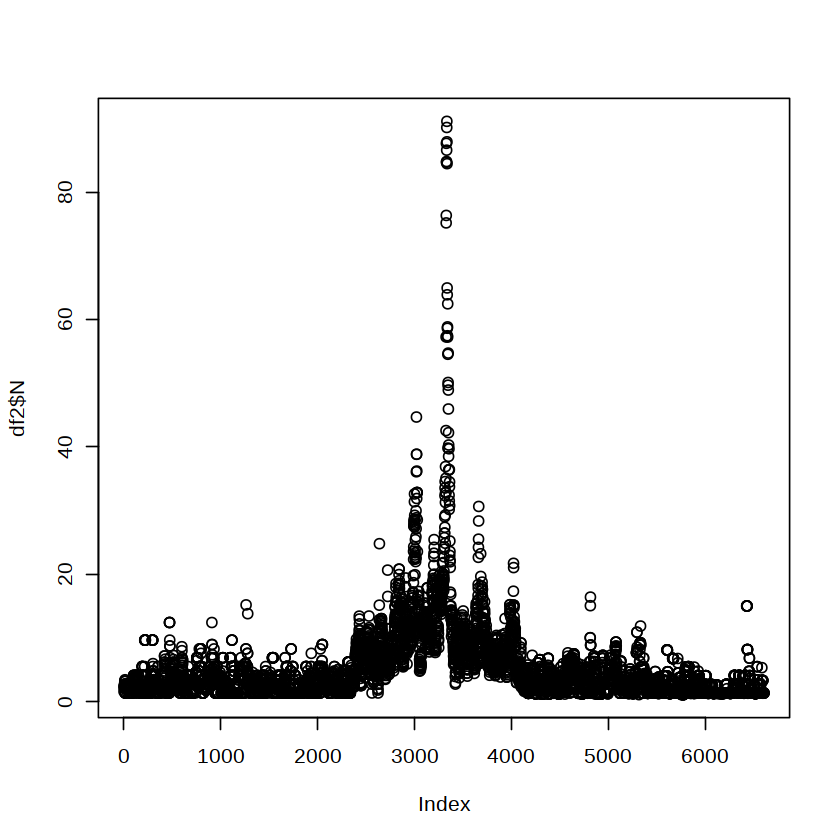
[6]:

plot(df2$N)

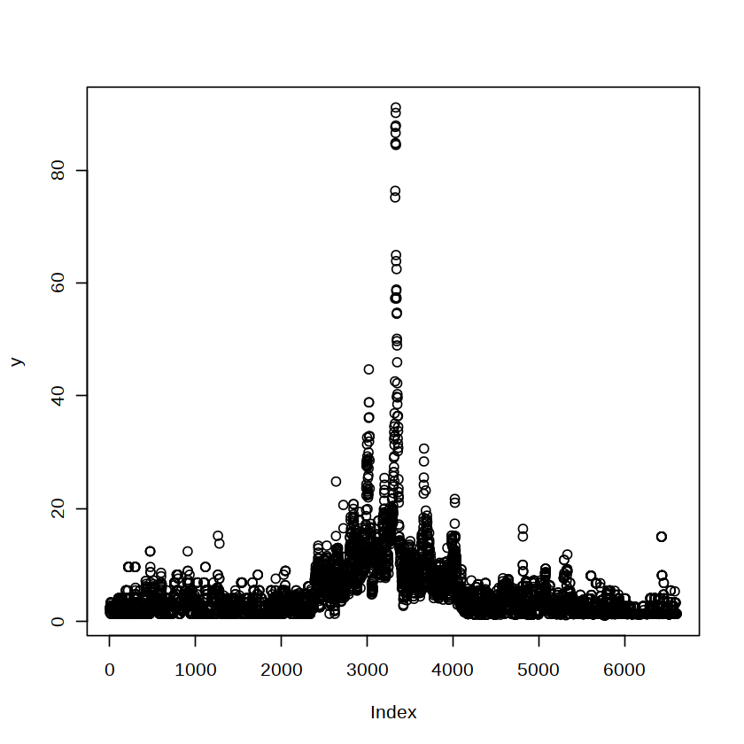
../_images/jupyter_notebooks_ChiCMaxima_algorithm_review_4_0.png

[10]:

y=df2[,"N"]
x=df2[,"start_OE"]
n <- length(y)
span=0.05
y.smooth <- loess(y ~ x, span=span)$fitted

[11]:

plot(y)

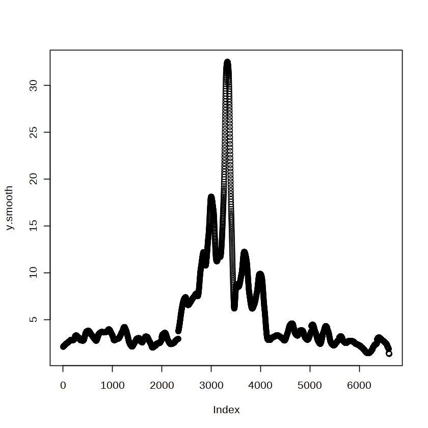
../_images/jupyter_notebooks_ChiCMaxima_algorithm_review_6_0.png

[12]:

plot(y.smooth)

../_images/jupyter_notebooks_ChiCMaxima_algorithm_review_7_0.png

[14]:

library(zoo)


Attaching package: ‘zoo’


The following objects are masked from ‘package:base’:

    as.Date, as.Date.numeric

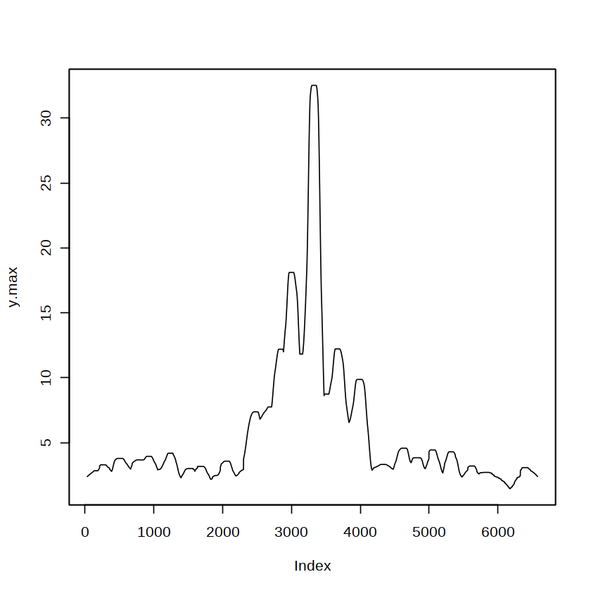
[16]:

w=30
y.max <- rollapply(zoo(y.smooth), 2*w+1,max,align="center")

[17]:

plot(y.max)

../_images/jupyter_notebooks_ChiCMaxima_algorithm_review_10_0.png

[18]:

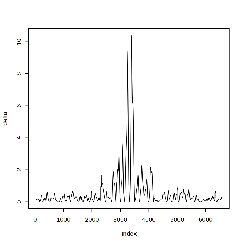
delta <- y.max - y.smooth[-c(1:w, n+1-1:w)]

[19]:

plot(delta)

../_images/jupyter_notebooks_ChiCMaxima_algorithm_review_12_0.png

[20]:

d=0
i.max <- which(delta <= d) + w

[29]:

?rollapply

rollapply {zoo}

R Documentation

Apply Rolling Functions

Description

A generic function for applying a function to rolling margins of an array.

Usage

rollapply(data, ...)
## S3 method for class 'ts'
rollapply(data, ...)
## S3 method for class 'zoo'
rollapply(data, width, FUN, ..., by = 1, by.column = TRUE,
    fill = if (na.pad) NA, na.pad = FALSE, partial = FALSE,
    align = c("center", "left", "right"), coredata = TRUE)
## Default S3 method:
rollapply(data, ...)
rollapplyr(..., align = "right")

Arguments

`data`	the data to be used (representing a series of observations).
`width`	numeric vector or list. In the simplest case this is an integer specifying the window width (in numbers of observations) which is aligned to the original sample according to the `align` argument. Alternatively, `width` can be a list regarded as offsets compared to the current time, see below for details.
`FUN`	the function to be applied.
`...`	optional arguments to `FUN`.
`by`	calculate FUN at every `by`-th time point rather than every point. `by` is only used if `width` is length 1 and either a plain scalar or a list.
`by.column`	logical. If `TRUE`, `FUN` is applied to each column separately.
`fill`	a three-component vector or list (recycled otherwise) providing filling values at the left/within/to the right of the data range. See the `fill` argument of `na.fill` for details.
`na.pad`	deprecated. Use `fill = NA` instead of `na.pad = TRUE`.
`partial`	logical or numeric. If `FALSE` (default) then `FUN` is only applied when all indexes of the rolling window are within the observed time range. If `TRUE`, then the subset of indexes that are in range are passed to `FUN`. A numeric argument to `partial` can be used to determin the minimal window size for partial computations. See below for more details.
`align`	specifyies whether the index of the result should be left- or right-aligned or centered (default) compared to the rolling window of observations. This argument is only used if `width` represents widths.
`coredata`	logical. Should only the `coredata(data)` be passed to every `width` window? If set to `FALSE` the full zoo series is used.

Details

If width is a plain numeric vector its elements are regarded as widths to be interpreted in conjunction with align whereas if width is a list its components are regarded as offsets. In the above cases if the length of width is 1 then width is recycled for every by-th point. If width is a list its components represent integer offsets such that the i-th component of the list refers to time points at positions i + width[[i]]. If any of these points are below 1 or above the length of index(data) then FUN is not evaluated for that point unless partial = TRUE and in that case only the valid points are passed.

The rolling function can also be applied to partial windows by setting partial = TRUE For example, if width = 3, align = "right" then for the first point just that point is passed to FUN since the two points to its left are out of range. For the same example, if partial = FALSE then FUN is not invoked at all for the first two points. If partial is a numeric then it specifies the minimum number of offsets that must be within range. Negative partial is interpreted as FALSE.

If width is a scalar then partial = TRUE and fill = NA are mutually exclusive but if offsets are specified for the width and 0 is not among the offsets then the output will be shorter than the input even if partial = TRUE is specified. In that case it may still be useful to specify fill in addition to partial.

If FUN is mean, max or median and by.column is TRUE and width is a plain scalar and there are no other arguments then special purpose code is used to enhance performance. Also in the case of mean such special purpose code is only invoked if the data argument has no NA values. See rollmean, rollmax and rollmedian for more details.

Currently, there are methods for "zoo" and "ts" series and "default" method for ordinary vectors and matrices.

rollapplyr is a wrapper around rollapply that uses a default of align = "right".

If data is of length 0, data is returned unmodified.

Value

A object of the same class as data with the results of the rolling function.

Examples

suppressWarnings(RNGversion("3.5.0"))
set.seed(1)

## rolling mean
z <- zoo(11:15, as.Date(31:35))
rollapply(z, 2, mean)

## non-overlapping means
z2 <- zoo(rnorm(6))
rollapply(z2, 3, mean, by = 3)      # means of nonoverlapping groups of 3
aggregate(z2, c(3,3,3,6,6,6), mean) # same

## optimized vs. customized versions
rollapply(z2, 3, mean)   # uses rollmean which is optimized for mean
rollmean(z2, 3)          # same
rollapply(z2, 3, (mean)) # does not use rollmean


## rolling regression:
## set up multivariate zoo series with
## number of UK driver deaths and lags 1 and 12
seat <- as.zoo(log(UKDriverDeaths))
time(seat) <- as.yearmon(time(seat))
seat <- merge(y = seat, y1 = lag(seat, k = -1),
  y12 = lag(seat, k = -12), all = FALSE)

## run a rolling regression with a 3-year time window
## (similar to a SARIMA(1,0,0)(1,0,0)_12 fitted by OLS)
rr <- rollapply(seat, width = 36,
  FUN = function(z) coef(lm(y ~ y1 + y12, data = as.data.frame(z))),
  by.column = FALSE, align = "right")

## plot the changes in coefficients
## showing the shifts after the oil crisis in Oct 1973
## and after the seatbelt legislation change in Jan 1983
plot(rr)


## rolling mean by time window (e.g., 3 days) rather than
## by number of observations (e.g., when these are unequally spaced):
#
## - test data
tt <- as.Date("2000-01-01") + c(1, 2, 5, 6, 7, 8, 10)
z <- zoo(seq_along(tt), tt)
## - fill it out to a daily series, zm, using NAs
## using a zero width zoo series g on a grid
g <- zoo(, seq(start(z), end(z), "day"))
zm <- merge(z, g)
## - 3-day rolling mean
rollapply(zm, 3, mean, na.rm = TRUE, fill = NA)
##
## - without expansion to regular grid: find interval widths
## that encompass the previous 3 days for each Date
w <- seq_along(tt) - findInterval(tt - 3, tt)
## a solution to computing the widths 'w' that is easier to read but slower
## w <- sapply(tt, function(x) sum(tt >= x - 2 & tt <= x))
##
## - rolling sum from 3-day windows
## without vs. with expansion to regular grid
rollapplyr(z, w, sum)
rollapplyr(zm, 3, sum, partial = TRUE, na.rm = TRUE)


## rolling weekly sums (with some missing dates)
z <- zoo(1:11, as.Date("2016-03-09") + c(0:7, 9:10, 12))
weeksum <- function(z) sum(z[time(z) > max(time(z)) - 7])
zs <- rollapplyr(z, 7, weeksum, fill = NA, coredata = FALSE)
merge(value = z, weeksum = zs)


## replicate cumsum with either 'partial' or vector width 'k'
cumsum(1:10)
rollapplyr(1:10, 10, sum, partial = TRUE)
rollapplyr(1:10, 1:10, sum)


## different values of rule argument
z <- zoo(c(NA, NA, 2, 3, 4, 5, NA))
rollapply(z, 3, sum, na.rm = TRUE)
rollapply(z, 3, sum, na.rm = TRUE, fill = NULL)
rollapply(z, 3, sum, na.rm = TRUE, fill = NA)
rollapply(z, 3, sum, na.rm = TRUE, partial = TRUE)

# this will exclude time points 1 and 2
# It corresponds to align = "right", width = 3
rollapply(zoo(1:8), list(seq(-2, 0)), sum)

# but this will include points 1 and 2
rollapply(zoo(1:8), list(seq(-2, 0)), sum, partial = 1)
rollapply(zoo(1:8), list(seq(-2, 0)), sum, partial = 0)

# so will this
rollapply(zoo(1:8), list(seq(-2, 0)), sum, fill = NA)

# by = 3, align = "right"
L <- rep(list(NULL), 8)
L[seq(3, 8, 3)] <- list(seq(-2, 0))
str(L)
rollapply(zoo(1:8), L, sum)

rollapply(zoo(1:8), list(0:2), sum, fill = 1:3)
rollapply(zoo(1:8), list(0:2), sum, fill = 3)

L2 <- rep(list(-(2:0)), 10)
L2[5] <- list(NULL)
str(L2)
rollapply(zoo(1:10), L2, sum, fill = "extend")
rollapply(zoo(1:10), L2, sum, fill = list("extend", NULL))

rollapply(zoo(1:10), L2, sum, fill = list("extend", NA))

rollapply(zoo(1:10), L2, sum, fill = NA)
rollapply(zoo(1:10), L2, sum, fill = 1:3)
rollapply(zoo(1:10), L2, sum, partial = TRUE)
rollapply(zoo(1:10), L2, sum, partial = TRUE, fill = 99)

rollapply(zoo(1:10), list(-1), sum, partial = 0)
rollapply(zoo(1:10), list(-1), sum, partial = TRUE)

rollapply(zoo(cbind(a = 1:6, b = 11:16)), 3, rowSums, by.column = FALSE)

# these two are the same
rollapply(zoo(cbind(a = 1:6, b = 11:16)), 3, sum)
rollapply(zoo(cbind(a = 1:6, b = 11:16)), 3, colSums, by.column = FALSE)

# these two are the same
rollapply(zoo(1:6), 2, sum, by = 2, align = "right")
aggregate(zoo(1:6), c(2, 2, 4, 4, 6, 6), sum)

# these two are the same
rollapply(zoo(1:3), list(-1), c)
lag(zoo(1:3), -1)

# these two are the same
rollapply(zoo(1:3), list(1), c)
lag(zoo(1:3))

# these two are the same
rollapply(zoo(1:5), list(c(-1, 0, 1)), sum)
rollapply(zoo(1:5), 3, sum)

# these two are the same
rollapply(zoo(1:5), list(0:2), sum)
rollapply(zoo(1:5), 3, sum, align = "left")

# these two are the same
rollapply(zoo(1:5), list(-(2:0)), sum)
rollapply(zoo(1:5), 3, sum, align = "right")

# these two are the same
rollapply(zoo(1:6), list(NULL, NULL, -(2:0)), sum)
rollapply(zoo(1:6), 3, sum, by = 3, align = "right")

# these two are the same
rollapply(zoo(1:5), list(c(-1, 1)), sum)
rollapply(zoo(1:5), 3, function(x) sum(x[-2]))

# these two are the same
rollapply(1:5, 3, rev)
embed(1:5, 3)

# these four are the same
x <- 1:6
rollapply(c(0, 0, x), 3, sum, align = "right") - x
rollapply(x, 3, sum, partial = TRUE, align = "right") - x
rollapply(x, 3, function(x) sum(x[-3]), partial = TRUE, align = "right")
rollapply(x, list(-(2:1)), sum, partial = 0)

# same as Matlab's buffer(x, n, p) for valid non-negative p
# See http://www.mathworks.com/help/toolbox/signal/buffer.html
x <- 1:30; n <- 7; p <- 3
t(rollapply(c(rep(0, p), x, rep(0, n-p)), n, by = n-p, c))

# these three are the same
y <- 10 * seq(8); k <- 4; d <- 2
# 1
# from http://ucfagls.wordpress.com/2011/06/14/embedding-a-time-series-with-time-delay-in-r-part-ii/
Embed <- function(x, m, d = 1, indices = FALSE, as.embed = TRUE) {
    n <- length(x) - (m-1)*d
    X <- seq_along(x)
    if(n <= 0)
        stop("Insufficient observations for the requested embedding")
    out <- matrix(rep(X[seq_len(n)], m), ncol = m)
    out[,-1] <- out[,-1, drop = FALSE] +
        rep(seq_len(m - 1) * d, each = nrow(out))
    if(as.embed)
        out <- out[, rev(seq_len(ncol(out)))]
    if(!indices)
        out <- matrix(x[out], ncol = m)
    out
}
Embed(y, k, d)
# 2
rollapply(y, list(-d * seq(0, k-1)), c)
# 3
rollapply(y, d*k-1, function(x) x[d * seq(k-1, 0) + 1])


## mimic convolve() using rollapplyr()
A <- 1:4
B <- 5:8
## convolve(..., type = "open")
cross <- function(x) x
rollapplyr(c(A, 0*B[-1]), length(B), cross, partial = TRUE)
convolve(A, B, type = "open")

# convolve(..., type = "filter")
rollapplyr(A, length(B), cross)
convolve(A, B, type = "filter")


# weighted sum including partials near ends, keeping
## alignment with wts correct
points <- zoo(cbind(lon = c(11.8300715, 11.8296697,
    11.8268708, 11.8267236, 11.8249612, 11.8251062),
  lat = c(48.1099048, 48.10884, 48.1067431, 48.1066077,
    48.1037673, 48.103318),
  dist = c(46.8463805878941, 33.4921440879536, 10.6101735030534,
    18.6085009578724, 6.97253109610173, 9.8912817449265)))
mysmooth <- function(z, wts = c(0.3, 0.4, 0.3)) {
  notna <- !is.na(z)
  sum(z[notna] * wts[notna]) / sum(wts[notna])
}
points2 <- points
points2[, 1:2] <- rollapply(rbind(NA, coredata(points)[, 1:2], NA), 3, mysmooth)
points2

[Package zoo version 1.8-10 ]

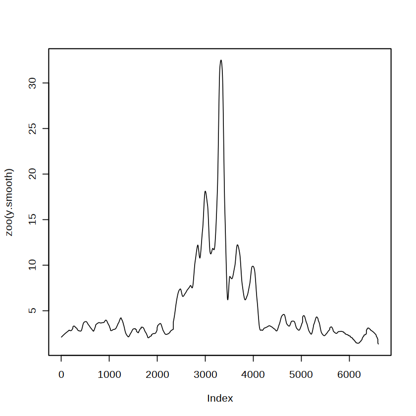
[28]:

plot(zoo(y.smooth))

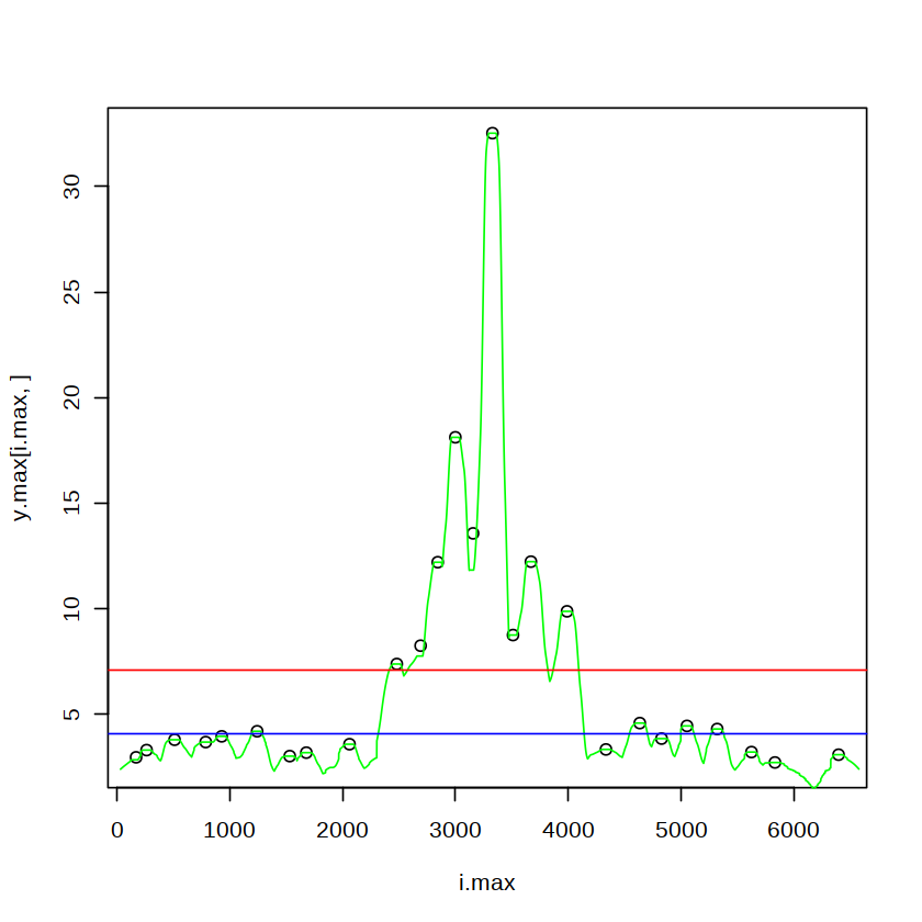
../_images/jupyter_notebooks_ChiCMaxima_algorithm_review_15_0.png

[38]:

plot(x=i.max,y=y.max[i.max,])
lines(y.max,col="green")
abline(h=median(y.max[i.max,]),col="blue")
abline(h=mean(y.max[i.max,]),col="red")

../_images/jupyter_notebooks_ChiCMaxima_algorithm_review_16_0.png

[37]:

?abline

abline {graphics}

R Documentation

Add Straight Lines to a Plot

Description

This function adds one or more straight lines through the current plot.

Usage

abline(a = NULL, b = NULL, h = NULL, v = NULL, reg = NULL,
       coef = NULL, untf = FALSE, ...)

Arguments

`a, b`	the intercept and slope, single values.
`untf`	logical asking whether to untransform. See ‘Details’.
`h`	the y-value(s) for horizontal line(s).
`v`	the x-value(s) for vertical line(s).
`coef`	a vector of length two giving the intercept and slope.
`reg`	an object with a `coef` method. See ‘Details’.
`...`	graphical parameters such as `col`, `lty` and `lwd` (possibly as vectors: see ‘Details’) and `xpd` and the line characteristics `lend`, `ljoin` and `lmitre`.

Details

Typical usages are

abline(a, b, untf = FALSE, \dots)
abline(h =, untf = FALSE, \dots)
abline(v =, untf = FALSE, \dots)
abline(coef =, untf = FALSE, \dots)
abline(reg =, untf = FALSE, \dots)

The first form specifies the line in intercept/slope form (alternatively a can be specified on its own and is taken to contain the slope and intercept in vector form).

The h= and v= forms draw horizontal and vertical lines at the specified coordinates.

The coef form specifies the line by a vector containing the slope and intercept.

reg is a regression object with a coef method. If this returns a vector of length 1 then the value is taken to be the slope of a line through the origin, otherwise, the first 2 values are taken to be the intercept and slope.

If untf is true, and one or both axes are log-transformed, then a curve is drawn corresponding to a line in original coordinates, otherwise a line is drawn in the transformed coordinate system. The h and v parameters always refer to original coordinates.

The graphical parameters col, lty and lwd can be specified; see par for details. For the h= and v= usages they can be vectors of length greater than one, recycled as necessary.

Specifying an xpd argument for clipping overrides the global par("xpd") setting used otherwise.

References

Becker, R. A., Chambers, J. M. and Wilks, A. R. (1988) The New S Language. Wadsworth & Brooks/Cole.

Murrell, P. (2005) R Graphics. Chapman & Hall/CRC Press.

Examples

## Setup up coordinate system (with x == y aspect ratio):
plot(c(-2,3), c(-1,5), type = "n", xlab = "x", ylab = "y", asp = 1)
## the x- and y-axis, and an integer grid
abline(h = 0, v = 0, col = "gray60")
text(1,0, "abline( h = 0 )", col = "gray60", adj = c(0, -.1))
abline(h = -1:5, v = -2:3, col = "lightgray", lty = 3)
abline(a = 1, b = 2, col = 2)
text(1,3, "abline( 1, 2 )", col = 2, adj = c(-.1, -.1))

## Simple Regression Lines:
require(stats)
sale5 <- c(6, 4, 9, 7, 6, 12, 8, 10, 9, 13)
plot(sale5)
abline(lsfit(1:10, sale5))
abline(lsfit(1:10, sale5, intercept = FALSE), col = 4) # less fitting

z <- lm(dist ~ speed, data = cars)
plot(cars)
abline(z) # equivalent to abline(reg = z) or
abline(coef = coef(z))

## trivial intercept model
abline(mC <- lm(dist ~ 1, data = cars)) ## the same as
abline(a = coef(mC), b = 0, col = "blue")

[Package graphics version 4.0.5 ]

ChiCMaxima algorithm review¶

Apply Rolling Functions

Description

Usage

Arguments

Details

Value

See Also

Examples

Add Straight Lines to a Plot

Description

Usage

Arguments

Details

References

See Also

Examples