What is MA plot?

MA plot shows the log average (A) on the -axis and the log ratio (M) on the -axis. Here, M stands for minus because

Similar plots are Bland-Altman plot, Tukey mean-difference plot, mean-difference plot, or MD plot.

This type of plot is good to show the data distribution between two individuals or two groups. Examples include:

• show data distribution in two replicates or two groups to identify systematic bias (if normalization is needed)

• show gene expression distribution comparing A to B, potentially highlighting differentially expressed genes, and/or other gene categories such as housekeeping genes, highly variable genes.

import pandas as pd
import matplotlib.pylab as plt
import seaborn as sns

df = pd.read_csv("/home/yli11/tmp/results.KO_vs_WT.csv",sep="\t",index_col=0)
df.head()

	logFC	AveExpr	t	P.Value	adj.P.Val	B	WT_1_log2CPM	WT_2_log2CPM	WT_3_log2CPM	KO_1_log2CPM	KO_2_log2CPM	KO_3_log2CPM
gene
D17H6S56E-5	-3.0830	9.3418	-97.669	2.276800e-15	3.597600e-11	25.102	10.8880	10.9120	10.8500	7.7671	7.8119	7.8218
Scd1	-2.2133	6.1060	-50.068	1.151200e-12	9.095200e-09	19.799	7.2574	7.1911	7.1920	5.0828	4.9264	4.9864
Coro2a	-1.4558	7.9154	-46.998	2.073900e-12	1.092300e-08	19.285	8.6433	8.6614	8.6256	7.1924	7.2202	7.1495
Plxnb2	-2.9373	3.6346	-42.033	5.854300e-12	1.598600e-08	17.639	5.0743	5.1443	5.1107	2.2122	2.2622	2.0040
Gzmb	-1.8469	4.9198	-41.606	6.436800e-12	1.598600e-08	18.097	5.7934	5.8635	5.8686	3.9655	3.9610	4.0665

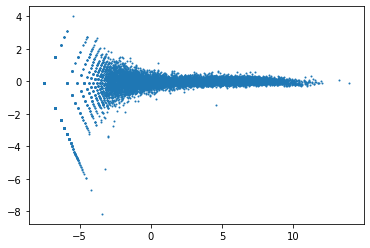
compare between replicates

A = (df['WT_1_log2CPM']+df['WT_2_log2CPM'])/2
M = df['WT_1_log2CPM']-df['WT_2_log2CPM']
plt.scatter(x=A,y=M,s=1) # s is point size

<matplotlib.collections.PathCollection at 0x2aad8f7f0280>

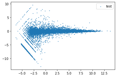
compare between two samples from different group

A = (df['WT_1_log2CPM']+df['KO_1_log2CPM'])/2
M = df['WT_1_log2CPM']-df['KO_1_log2CPM']
plt.scatter(x=A,y=M,s=1) # s is point size
plt.legend(["test"])

<matplotlib.legend.Legend at 0x2aad901dd6a0>

compare between groups

# extract column names, you can also just type column names manually
WT_column_names = [x for x in df.columns if "WT" in x] # When using only 'if', put 'for' in the beginning
KO_column_names = [x for x in df.columns if "KO" in x] # When using only 'if', put 'for' in the beginning
print (WT_column_names)
print (KO_column_names)

['WT_1_log2CPM', 'WT_2_log2CPM', 'WT_3_log2CPM']
['KO_1_log2CPM', 'KO_2_log2CPM', 'KO_3_log2CPM']

a=[1,2,3,"asd"]
a

[1, 2, 3, 'asd']

list(range(0,10))

[0, 1, 2, 3, 4, 5, 6, 7, 8, 9]

[i/2 for i in range(0,10)]

[0.0, 0.5, 1.0, 1.5, 2.0, 2.5, 3.0, 3.5, 4.0, 4.5]

output = []
for i in range(0,10):
    output.append(i/2)
output

[0.0, 0.5, 1.0, 1.5, 2.0, 2.5, 3.0, 3.5, 4.0, 4.5]

df.columns

Index(['logFC', 'AveExpr', 't', 'P.Value', 'adj.P.Val', 'B', 'WT_1_log2CPM',
       'WT_2_log2CPM', 'WT_3_log2CPM', 'KO_1_log2CPM', 'KO_2_log2CPM',
       'KO_3_log2CPM'],
      dtype='object')

df.shape

(15801, 12)

[i for i in df.columns if "W" in i]

['WT_1_log2CPM', 'WT_2_log2CPM', 'WT_3_log2CPM']

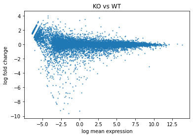
A = (df[WT_column_names].mean(axis=1)+df[KO_column_names].mean(axis=1))/2
M = df[KO_column_names].mean(axis=1)-df[WT_column_names].mean(axis=1)
plt.scatter(x=A,y=M,s=1) # s is point size
## add cosmetics
plt.title("KO vs WT")
plt.xlabel("log mean expression")
plt.ylabel("log fold change")

Text(0, 0.5, 'log fold change')

df.head()

	logFC	AveExpr	t	P.Value	adj.P.Val	B	WT_1_log2CPM	WT_2_log2CPM	WT_3_log2CPM	KO_1_log2CPM	KO_2_log2CPM	KO_3_log2CPM
gene
D17H6S56E-5	-3.0830	9.3418	-97.669	2.276800e-15	3.597600e-11	25.102	10.8880	10.9120	10.8500	7.7671	7.8119	7.8218
Scd1	-2.2133	6.1060	-50.068	1.151200e-12	9.095200e-09	19.799	7.2574	7.1911	7.1920	5.0828	4.9264	4.9864
Coro2a	-1.4558	7.9154	-46.998	2.073900e-12	1.092300e-08	19.285	8.6433	8.6614	8.6256	7.1924	7.2202	7.1495
Plxnb2	-2.9373	3.6346	-42.033	5.854300e-12	1.598600e-08	17.639	5.0743	5.1443	5.1107	2.2122	2.2622	2.0040
Gzmb	-1.8469	4.9198	-41.606	6.436800e-12	1.598600e-08	18.097	5.7934	5.8635	5.8686	3.9655	3.9610	4.0665

hk_genes = HemData.get_housekeeping_genes()
hk_genes

/home/yli11/.conda/envs/captureC/lib/python3.8/site-packages/HemTools/HemData.py:11: ParserWarning: Falling back to the 'python' engine because the 'c' engine does not support regex separators (separators > 1 char and different from '\s+' are interpreted as regex); you can avoid this warning by specifying engine='python'.
  names = pd.read_csv(f"{pdir}/../HemData/index.tsv", sep="\s", header=None, index_col=0)[1].to_dict()

	Mouse	Human
0	1600012H06Rik	C6orf120
1	1700123O20Rik	C14orf119
2	1810009A15Rik	C11orf98
3	1810013L24Rik	C16orf72
4	2610507B11Rik	KIAA0100
...	...	...
1125	Zmynd19	ZMYND19
1126	Zranb1	ZRANB1
1127	Zranb2	ZRANB2
1128	Zrsr1	ZRSR2
1129	Zyg11b	ZYG11B

1130 rows × 2 columns

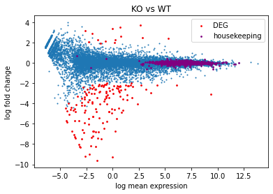
A = (df[WT_column_names].mean(axis=1)+df[KO_column_names].mean(axis=1))/2
M = df[KO_column_names].mean(axis=1)-df[WT_column_names].mean(axis=1)
plt.scatter(x=A,y=M,s=1) # s is point size

# deg
deg = df[(df['logFC'].abs()>=2)&(df['adj.P.Val']<=0.01)]
degA = (deg[WT_column_names].mean(axis=1)+deg[KO_column_names].mean(axis=1))/2
degM = deg[KO_column_names].mean(axis=1)-deg[WT_column_names].mean(axis=1)
plt.scatter(x=degA,y=degM,s=3,color="red",label="DEG") # s is point size

from HemTools import HemData
hk_genes = HemData.get_housekeeping_genes()

# deg
hk = df.loc[df.index.intersection(hk_genes.Mouse)]
hkA = (hk[WT_column_names].mean(axis=1)+hk[KO_column_names].mean(axis=1))/2
hkM = hk[KO_column_names].mean(axis=1)-hk[WT_column_names].mean(axis=1)
plt.scatter(x=hkA,y=hkM,s=3,color="purple",label="housekeeping") # s is point size


## add cosmetics
plt.title("KO vs WT")
plt.xlabel("log mean expression")
plt.ylabel("log fold change")
plt.legend()

/home/yli11/.conda/envs/captureC/lib/python3.8/site-packages/HemTools/HemData.py:11: ParserWarning: Falling back to the 'python' engine because the 'c' engine does not support regex separators (separators > 1 char and different from '\s+' are interpreted as regex); you can avoid this warning by specifying engine='python'.
  names = pd.read_csv(f"{pdir}/../HemData/index.tsv", sep="\s", header=None, index_col=0)[1].to_dict()

<matplotlib.legend.Legend at 0x2aad9008ff10>

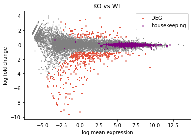
add more gene categories

• differentially expressed genes

• housekeeping genes

A = (df[WT_column_names].mean(axis=1)+df[KO_column_names].mean(axis=1))/2
M = df[KO_column_names].mean(axis=1)-df[WT_column_names].mean(axis=1)

deg = df[(df['logFC'].abs()>=1)&(df['adj.P.Val']<=0.01)]
# Tip: use Ctrl+D (Windows) or Command + D (Mac) to do multi-selection and replace
degA = (deg[WT_column_names].mean(axis=1)+deg[KO_column_names].mean(axis=1))/2
degM = deg[KO_column_names].mean(axis=1)-deg[WT_column_names].mean(axis=1)

from HemTools import HemData
hk_genes = HemData.get_housekeeping_genes()
hk = df.loc[df.index.intersection(hk_genes.Mouse)]
# Tip: use Ctrl+D (Windows) or Command + D (Mac) to do multi-selection and replace
hkA = (hk[WT_column_names].mean(axis=1)+hk[KO_column_names].mean(axis=1))/2
hkM = hk[KO_column_names].mean(axis=1)-hk[WT_column_names].mean(axis=1)


plt.scatter(x=A,y=M,s=1,color="grey") # s is point size
plt.scatter(x=degA,y=degM,s=3,color="#E64B35",label="DEG") # s is point size
plt.scatter(x=hkA,y=hkM,s=3,color="purple",label="housekeeping") # s is point size

## add cosmetics
plt.title("KO vs WT")
plt.xlabel("log mean expression")
plt.ylabel("log fold change")
plt.legend()

/home/yli11/.conda/envs/captureC/lib/python3.8/site-packages/HemTools/HemData.py:11: ParserWarning: Falling back to the 'python' engine because the 'c' engine does not support regex separators (separators > 1 char and different from '\s+' are interpreted as regex); you can avoid this warning by specifying engine='python'.
  names = pd.read_csv(f"{pdir}/../HemData/index.tsv", sep="\s", header=None, index_col=0)[1].to_dict()

<matplotlib.legend.Legend at 0x2aad8ffe1e50>