Volcano plot
Volcano plot is a scatter plot specifically for showing significant levels (e.g., p-value) and fold-changes
[3]:
import pandas as pd
import matplotlib.pylab as plt
import seaborn as sns
import numpy as np
[2]:
df = pd.read_csv("/home/yli11/tmp/results.KO_vs_WT.csv",sep="\t",index_col=0)
df.head()
[2]:
| logFC | AveExpr | t | P.Value | adj.P.Val | B | WT_1_log2CPM | WT_2_log2CPM | WT_3_log2CPM | KO_1_log2CPM | KO_2_log2CPM | KO_3_log2CPM | |
|---|---|---|---|---|---|---|---|---|---|---|---|---|
| gene | ||||||||||||
| D17H6S56E-5 | -3.0830 | 9.3418 | -97.669 | 2.276800e-15 | 3.597600e-11 | 25.102 | 10.8880 | 10.9120 | 10.8500 | 7.7671 | 7.8119 | 7.8218 |
| Scd1 | -2.2133 | 6.1060 | -50.068 | 1.151200e-12 | 9.095200e-09 | 19.799 | 7.2574 | 7.1911 | 7.1920 | 5.0828 | 4.9264 | 4.9864 |
| Coro2a | -1.4558 | 7.9154 | -46.998 | 2.073900e-12 | 1.092300e-08 | 19.285 | 8.6433 | 8.6614 | 8.6256 | 7.1924 | 7.2202 | 7.1495 |
| Plxnb2 | -2.9373 | 3.6346 | -42.033 | 5.854300e-12 | 1.598600e-08 | 17.639 | 5.0743 | 5.1443 | 5.1107 | 2.2122 | 2.2622 | 2.0040 |
| Gzmb | -1.8469 | 4.9198 | -41.606 | 6.436800e-12 | 1.598600e-08 | 18.097 | 5.7934 | 5.8635 | 5.8686 | 3.9655 | 3.9610 | 4.0665 |
[7]:
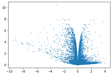
plt.scatter(x=df['logFC'],y=df['adj.P.Val'].apply(lambda x:-np.log10(x)),s=1)
[7]:
<matplotlib.collections.PathCollection at 0x2aad5daf8df0>
[13]:
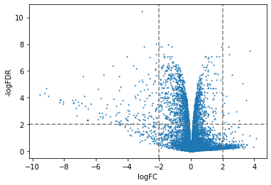
plt.scatter(x=df['logFC'],y=df['adj.P.Val'].apply(lambda x:-np.log10(x)),s=1)
plt.xlabel("logFC")
plt.ylabel("-logFDR")
plt.axvline(-2,color="grey",linestyle="--")
plt.axvline(2,color="grey",linestyle="--")
plt.axhline(2,color="grey",linestyle="--")
[13]:
<matplotlib.lines.Line2D at 0x2aad5dde57c0>
[16]:
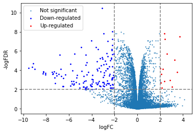
plt.scatter(x=df['logFC'],y=df['adj.P.Val'].apply(lambda x:-np.log10(x)),s=1,label="Not significant")

# highlight down- or up- regulated genes
down = df[(df['logFC']<=-2)&(df['adj.P.Val']<=0.01)]
up = df[(df['logFC']>=2)&(df['adj.P.Val']<=0.01)]

plt.scatter(x=down['logFC'],y=down['adj.P.Val'].apply(lambda x:-np.log10(x)),s=3,label="Down-regulated",color="blue")
plt.scatter(x=up['logFC'],y=up['adj.P.Val'].apply(lambda x:-np.log10(x)),s=3,label="Up-regulated",color="red")

plt.xlabel("logFC")
plt.ylabel("-logFDR")
plt.axvline(-2,color="grey",linestyle="--")
plt.axvline(2,color="grey",linestyle="--")
plt.axhline(2,color="grey",linestyle="--")
plt.legend()
[16]:
<matplotlib.legend.Legend at 0x2aad5e36fbe0>
[28]:
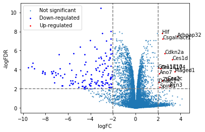
plt.scatter(x=df['logFC'],y=df['adj.P.Val'].apply(lambda x:-np.log10(x)),s=1,label="Not significant")

# highlight down- or up- regulated genes
down = df[(df['logFC']<=-2)&(df['adj.P.Val']<=0.01)]
up = df[(df['logFC']>=2)&(df['adj.P.Val']<=0.01)]

plt.scatter(x=down['logFC'],y=down['adj.P.Val'].apply(lambda x:-np.log10(x)),s=3,label="Down-regulated",color="blue")
plt.scatter(x=up['logFC'],y=up['adj.P.Val'].apply(lambda x:-np.log10(x)),s=3,label="Up-regulated",color="red")
for i,r in up.iterrows():
    plt.text(x=r['logFC'],y=-np.log10(r['adj.P.Val']),s=i)

plt.xlabel("logFC")
plt.ylabel("-logFDR")
plt.axvline(-2,color="grey",linestyle="--")
plt.axvline(2,color="grey",linestyle="--")
plt.axhline(2,color="grey",linestyle="--")
plt.legend()
[28]:
<matplotlib.legend.Legend at 0x2aad619b2700>
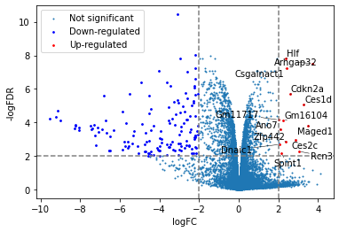
[31]:
from adjustText import adjust_text

plt.scatter(x=df['logFC'],y=df['adj.P.Val'].apply(lambda x:-np.log10(x)),s=1,label="Not significant")

# highlight down- or up- regulated genes
down = df[(df['logFC']<=-2)&(df['adj.P.Val']<=0.01)]
up = df[(df['logFC']>=2)&(df['adj.P.Val']<=0.01)]

plt.scatter(x=down['logFC'],y=down['adj.P.Val'].apply(lambda x:-np.log10(x)),s=3,label="Down-regulated",color="blue")
plt.scatter(x=up['logFC'],y=up['adj.P.Val'].apply(lambda x:-np.log10(x)),s=3,label="Up-regulated",color="red")
texts=[]
for i,r in up.iterrows():
    texts.append(plt.text(x=r['logFC'],y=-np.log10(r['adj.P.Val']),s=i))
adjust_text(texts,arrowprops=dict(arrowstyle="-", color='black', lw=0.5))
plt.xlabel("logFC")
plt.ylabel("-logFDR")
plt.axvline(-2,color="grey",linestyle="--")
plt.axvline(2,color="grey",linestyle="--")
plt.axhline(2,color="grey",linestyle="--")
plt.legend()
[31]:
<matplotlib.legend.Legend at 0x2aad61abe760>
[ ]: