Visualizing high-dimentional data using PCA or UMAP
usage: plot_PCA.py [-h] [-j JID] [--remove_zero] [--index] [--binarize]
                   [--max MAX] [--min MIN] [--transpose] [--sample_norm] -f
                   INPUT [--use_cols USE_COLS] [--index_using INDEX_USING]
                   [-s SEP] [--xlabel XLABEL] [--ylabel YLABEL]
                   [--remove_cols REMOVE_COLS]
                   [--color_using COLOR_USING | --color_by_a_col COLOR_BY_A_COL | --shape_by_str SHAPE_BY_STR]
                   [-n MAXPC] [--UMAP_min_dist UMAP_MIN_DIST]
                   [--UMAP_metric UMAP_METRIC]
                   [--UMAP_n_neighbors UMAP_N_NEIGHBORS] [--title TITLE]
                   [--label_by_last3_element] [--smart_label]
                   [--kmeans_label KMEANS_LABEL] [--dbscan_label]
                   [--guess_label] [--continous]
                   [--gene_filter_cutoff GENE_FILTER_CUTOFF]
                   [--label_by_first_element] [--label_by_first4_element]
                   [--zero_mean_unit_variance] [--label_by_meaningful_name]
                   [--UMAP] [--nPCA_UMAP NPCA_UMAP] [--text]
                   [--save_projection_df] [--figure_type FIGURE_TYPE]
                   [-o OUTPUT] [--header] [-W WIDTH] [-H HEIGHT]
                   [--log2_transform]

plot heatmap given dataframe.

optional arguments:
  -h, --help            show this help message and exit
  -j JID, --jid JID     enter a job ID, which is used to make a new directory.
                        Every output will be moved into this folder. (default:
                        plot_PCA_yli11_2020-09-03)
  --remove_zero         remove all rows or cols that are zero (default: False)
  --index               index is false (default: False)
  --binarize            force to binary data (default: False)
  --max MAX             above this value to determine 1 (default: 1)
  --min MIN             above this value to determine 0 (default: 0)
  --transpose           df transpose (default: False)
  --sample_norm         sample norm by sum (default: False)
  -f INPUT, --input INPUT
                        data table input (default: None)
  --use_cols USE_COLS   use a subset cols (default: None)
  --index_using INDEX_USING
                        Sometimes we want to show a different label for the
                        indices, then use this option. For example, gene id is
                        unique, however, gene name can be different, it also
                        has upper or lower case problem, in such case, we want
                        to use gene id for data processing and use gene name
                        for visualization. (default: )
  -s SEP, --sep SEP     separator (default: )
  --xlabel XLABEL
  --ylabel YLABEL
  --remove_cols REMOVE_COLS
  --color_using COLOR_USING
                        input a file, index should be the same as the input
                        data frame (default: None)
  --color_by_a_col COLOR_BY_A_COL
                        input a column name to be used for coloring (default:
                        None)
  --shape_by_str SHAPE_BY_STR
                        input a string to match sample name, matched and
                        unmatched names will have different name; used to show
                        our own data vs public data. (default: None)
  -n MAXPC, --maxPC MAXPC
  --UMAP_min_dist UMAP_MIN_DIST
  --UMAP_metric UMAP_METRIC
  --UMAP_n_neighbors UMAP_N_NEIGHBORS
  --title TITLE
  --label_by_last3_element
  --smart_label
  --kmeans_label KMEANS_LABEL
  --dbscan_label
  --guess_label
  --continous
  --gene_filter_cutoff GENE_FILTER_CUTOFF
  --label_by_first_element
  --label_by_first4_element
  --zero_mean_unit_variance
  --label_by_meaningful_name
  --UMAP
  --nPCA_UMAP NPCA_UMAP
  --text
  --save_projection_df
  --figure_type FIGURE_TYPE
                        pdf,png,jpeg (default: png)
  -o OUTPUT, --output OUTPUT
                        output table name (default: plot_PCA_yli11_2020-09-03)
  --header              input table has header (default: False)
  -W WIDTH, --width WIDTH
                        Figure width, by default, w=N_row/4, if given, will
                        replace the default value (default: 500)
  -H HEIGHT, --height HEIGHT
                        Figure height, by default, w=N_col/4, if given, will
                        replace the default value (default: 500)
  --log2_transform      input values will be log2 transformed (default: False)
Summary
Given a dataframe, make a PCA or UMAP plot.
Example
Input
Data table, tsv (default) or csv (-s ,). If data table contains both row names and column names, use --index --header
Usage
hpcf_interactive -q standard -R "rusage[mem=10000]"

module load conda3

source activate /home/yli11/.conda/envs/py2/
Example usage
plot_PCA.py -f /home/yli11/HemPortal/RNA_seq/erythopoesis_expr.transcript.tpm --index --header --transpose --label_by_first_element
Note that --index --header specifies that the input data has column names and row names.
In the input, we assume columns are used as features and rows are used as samples, in other words, the number of dots in the output figure is equal to the row names. (This is a general machine learning format.)
In the input example, the rows are actually the features, so I need to do a matrix transpose, use --transpose.
In the input example, we don’t have a label column, and we just want to use the row names as the label, use --label_by_first_element.
Usage-UMAP
Example usage
plot_PCA.py -f /home/yli11/HemPortal/RNA_seq/blood/combined_gene_exp/merged_gene_exp.tsv --UMAP --index --header --transpose
Or try different parameters:
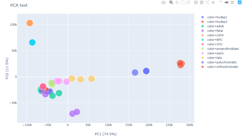
Output
This is an interactive figure, please open the html file.
Data exploration for machine learning projects
Input
Standard ML format uses row for individual samples/instances and column for individual features/predictors. There is another column for the labels if it is supervised learning.
Aim
Visualze the sample distribution given selected features.
Usage
hpcf_interactive -q standard -R "rusage[mem=10000]"

module load conda3

source activate /home/yli11/.conda/envs/py2/

plot_PCA.py -f input.csv --color_by_a_col label --header -s , --UMAP
FAQ
PCA plot for gene exp results from running diffgene.py or HemTools rna_seq
We will use tpm values calculated from Kallisto. This is stored in individual abandunce.tsv file. Go to your result dir and do the following
module load python/2.7.13

dataframe_merge.py --drop length,eff_length,est_counts --rename_col_with_filename -o merged_raw.tsv */*.tsv

dataframe.py --remove_zero --row --index --header -f merged_raw.tsv -o forPCA.tsv

module load conda3
source activate /home/yli11/.conda/envs/py2

plot_PCA.py -f forPCA.tsv --index --header --transpose --label_by_last3_element --log2_transform -o PCA_plot_log2TPM.html

plot_PCA.py -f forPCA.tsv --index --header --transpose --label_by_last3_element -o PCA_plot_TPM.html
Example 2: merge and plot
In my current working dir, I have downloaded GSE116177, where it has SE RNA-seq and PE RNA-seq, so I analysized them differently. I also have my own data. The first step is to find the output from HemTools_dev rna_seq pipeline, shown below.
module load python/2.7.13

find . -name "rna_seq_yli11_2019*.gene.abundance.csv"

./GSE116177/renamed_data/single/rna_seq_yli11_2019-12-24/kallisto_files/rna_seq_yli11_2019-12-24.gene.abundance.csv

./GSE116177/renamed_data/paired/rna_seq_yli11_2019-12-24/kallisto_files/rna_seq_yli11_2019-12-24.gene.abundance.csv

./combine_129304_134393_140290/rna_seq_yli11_2019-12-24/kallisto_files/rna_seq_yli11_2019-12-24.gene.abundance.csv
Then merge the three datasets:
dataframe_merge.py ./GSE116177/renamed_data/single/rna_seq_yli11_2019-12-24/kallisto_files/rna_seq_yli11_2019-12-24.gene.abundance.csv ./GSE116177/renamed_data/paired/rna_seq_yli11_2019-12-24/kallisto_files/rna_seq_yli11_2019-12-24.gene.abundance.csv ./combine_129304_134393_140290/rna_seq_yli11_2019-12-30/kallisto_files/rna_seq_yli11_2019-12-30.gene.abundance.csv --intersection -o merged_rwu_GSE116177.tsv --drop "Gene Name"

dataframe_merge.py ./GSE116177/renamed_data/single/rna_seq_yli11_2019-12-24/kallisto_files/rna_seq_yli11_2019-12-24.gene.abundance.csv ./GSE116177/renamed_data/paired/rna_seq_yli11_2019-12-24/kallisto_files/rna_seq_yli11_2019-12-24.gene.abundance.csv ./combine_129304_134393_140290/rna_seq_yli11_2019-12-30/kallisto_files/rna_seq_yli11_2019-12-30.gene.abundance.csv --intersection -o merged_rwu_GSE116177_with_gene_name.tsv
Lastly make a UMAP plot:
module load conda3
source activate /home/yli11/.conda/envs/py2

plot_PCA.py -f merged_rwu_GSE116177.tsv --index --header --transpose --log2_transform  --UMAP -o scaled_UMAP_log2TPM_filtered.html --smart_label --gene_filter_cutoff 1 --shape_by_str GSM --zero_mean_unit_variance
Parameters in UMAP
Number of clusters
less UMAP_min_dist and less number of neighbors will give more clusters.
UMAP_n_neighbors will have less impact when UMAP_min_dist <=0.1
Range of UMAP_min_dist depends on the distance matrics. In most cases, you just need to pick a value from 0 to 1.
Comments
code @ github.