Uditas
Summary
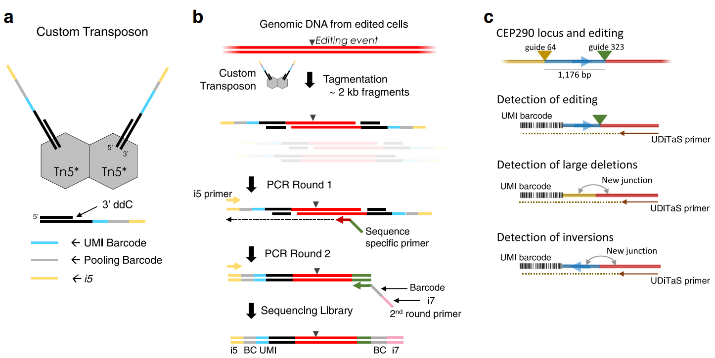
UDiTaS (UniDirectional Targeted Sequencing) is a method to capture indels and structural rearrangements.
12/5/2022 updates
Original code is optimized, see: https://github.com/YichaoOU/uditas_opt
Input
A folder that contains:
Undetermined_S0_R1_001.fastq.gz
Undetermined_S0_R2_001.fastq.gz
Undetermined_S0_I1_001.fastq.gz
Undetermined_S0_I2_001.fastq.gz
sample_info.csv
sample_info.csv this file name is fixed, the name has to be exactly the same. Format can be found here: https://github.com/editasmedicine/uditas/blob/master/data/fig2c/sample_info.csv
NEW: add gRNA info to control samples.
Fastq file names have to be exactly the same.
Usage
prepare input.list, 0-based row index. For example, if we have 6 samples in
sample_info.csv, then the input.list will look like below.
head input.list
--------------
0
1
2
3
4
5
go to the working dir and run the following [submit job].
hpcf_interactive

module load python/2.7.13

run_lsf.py -f input.list -p uditas_opt
Output
Raw reads are first demultiplexed, the overall demultiplexing rate should > 90%. See
reports/report_overall.xls.Then reads are trimmed, how many reads are left? See
multiqc_report.html, you need to run multiQC yourself (outside stjude).Then reads are local aligned to the genome, what is the alignment rate, should > 90%. See
multiqc_report.html.Then reads are mapped to the amplicons, what is the total number of junction reads? See
reports/total_collapsed_junction_reads.csv. Details of each amplicon mapped reads can be found in$sample_name/bam_amplicon_files/*amplicon_mapping.tsv.For reads that can’t be mapped to the amplicons, they are global aligned to the genome, the mapping rate is an indicator for mis-priming events. See
multiqc_report.html.SV frequency heatmap and circos plot are generated using
heatmap_circos_plot.ipynb
UDITAS pipeline notes
These notes are mainly for me to better understand the code.
The pipeline creates results for each sample, stored in the sample name folder. They have a
only_summarizeoption so that I can run UDITAS pipeline for each sample (so as to parallize the pipeline) and then once everything is finished, run the summarize function.
Steps
Demultiplexing: based on hamming distance, allowing for 1 mismatch. Stats stored in
reportsfolder
Double cut senarios, cut is -3 (hardcoded, for NGG cas9):
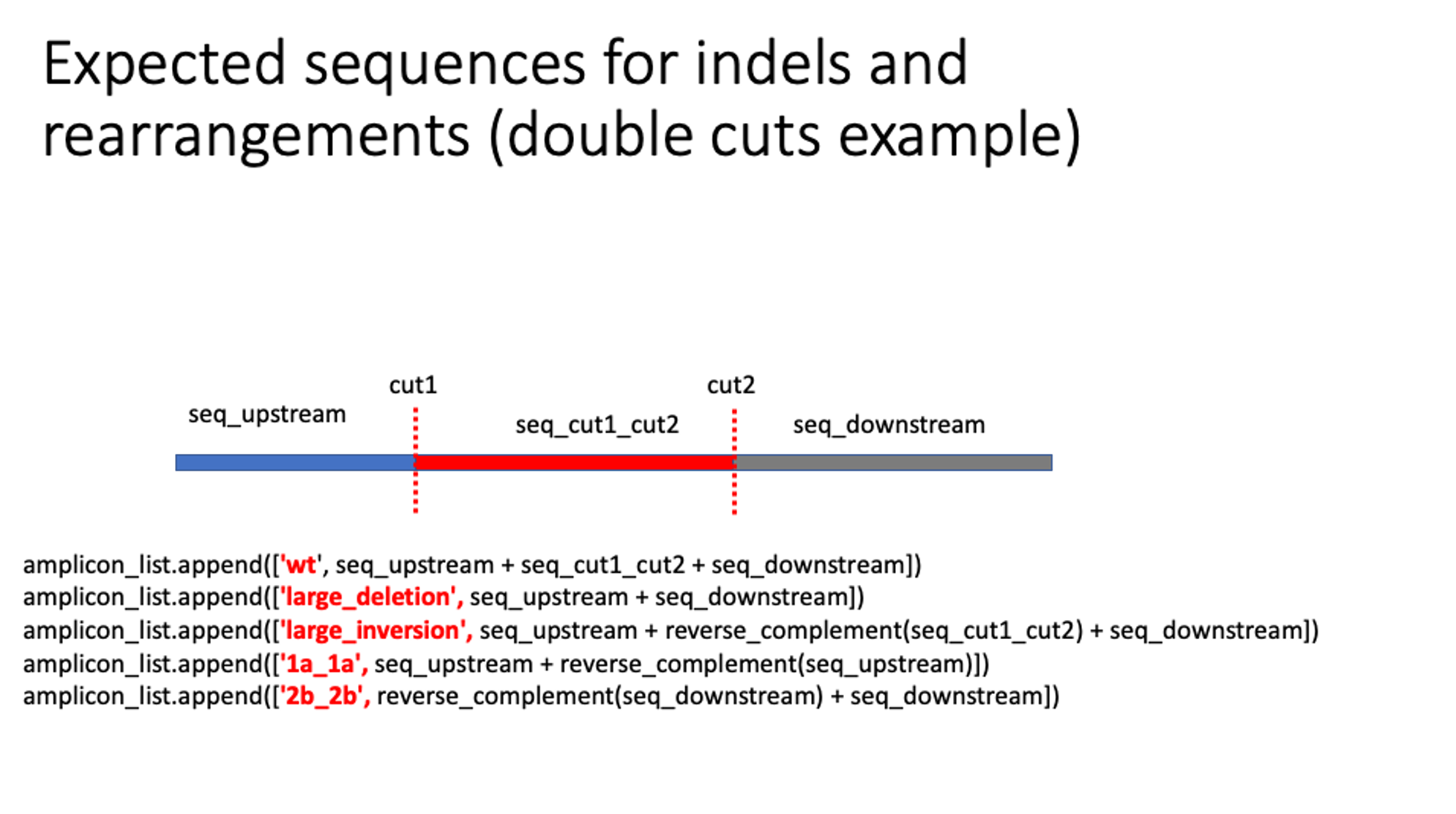
# amplicon_window_around_cut default 1kb
start_coordinate = int(cut1 - amplicon_window_around_cut)
end_coordinate = int(cut2 + amplicon_window_around_cut)
# We switch the coordinates of cut1 and cut2 if the guides are provided so that cut2 < cut1
seq_upstream = genome[amplicon_info['chr_guide_1']][start_coordinate:int(cut1)]
seq_cut1_cut2 = genome[amplicon_info['chr_guide_1']][int(cut1):int(cut2)]
seq_downstream = genome[amplicon_info['chr_guide_1']][int(cut2):end_coordinate]

amplicon_list.append(['wt', seq_upstream + seq_cut1_cut2 + seq_downstream])
amplicon_list.append(['large_deletion', seq_upstream + seq_downstream])
amplicon_list.append(['large_inversion', seq_upstream + reverse_complement(seq_cut1_cut2) + seq_downstream])
amplicon_list.append(['1a_1a', seq_upstream + reverse_complement(seq_upstream)])
amplicon_list.append(['2b_2b', reverse_complement(seq_downstream) + seq_downstream])
A note on preparing sample_info.csv
Many columns are not used, such as: NGS_req-ID, name, Sample, description, Control sample (Y/N), Cell name_type, etc.
Sample info.csv supports upto 3 cuts, which are guide_1, guide_2, and guide_3 columns. Fill in as needed.
plasmid_sequence for plasmid-based experiments
Replicate figure 2C
It took me a while to find the actual primer name for each SRA ID because it was not provided in the SRA metadata file.
Run,Library Name,LibraryLayout,replicate,Antibody
SRR6704713,library_13_umi,SINGLE,biological replicate 2,OLI6256
SRR6704714,library_13,PAIRED,biological replicate 2,OLI6256
SRR6704715,library_14_umi,SINGLE,biological replicate 1,OLI6259
SRR6704716,library_14,PAIRED,biological replicate 1,OLI6259
SRR6704719,library_12_umi,SINGLE,biological replicate 1,OLI6256
SRR6704720,library_12,PAIRED,biological replicate 1,OLI6256
SRR6704721,library_15_umi,SINGLE,biological replicate 2,OLI6259
SRR6704722,library_15,PAIRED,biological replicate 2,OLI6259
Download data from SRA. /home/yli11/dirs/shengdar_group/users/Yichao/Uditas/PRJNA433666/sra_download_yli11_2022-06-06/names
UMI and R1/R2 have different read names, I have to preprocess them so that:
read name is the same
index1 and index2 contains sample barcode because the Uditas code must start from demultiplexing, otherwise you have to make sure the folder structure is the same to skip demultiplexing.
seq_1a = genome[amplicon_info['chr_guide_1']][start_coordinate1:int(cut1)]
seq_1b = genome[amplicon_info['chr_guide_1']][int(cut1):end_coordinate1]
seq_2a = genome[amplicon_info['chr_guide_2']][start_coordinate2:int(cut2)]
seq_2b = genome[amplicon_info['chr_guide_2']][int(cut2):end_coordinate2]

amplicon_list.append(['1a_1a', seq_1a + reverse_complement(seq_1a)])
amplicon_list.append(['1a_1b', seq_1a + seq_1b])
amplicon_list.append(['1a_2a', seq_1a + reverse_complement(seq_2a)])
amplicon_list.append(['1a_2b', seq_1a + seq_2b])

amplicon_list.append(['1b_1b', reverse_complement(seq_1b) + seq_1b])
amplicon_list.append(['2a_1b', seq_2a + seq_1b])
amplicon_list.append(['2b_1b', reverse_complement(seq_2b) + seq_1b])

amplicon_list.append(['2a_2a', seq_2a + reverse_complement(seq_2a)])
amplicon_list.append(['2a_2b', seq_2a + seq_2b])

amplicon_list.append(['2b_2b', reverse_complement(seq_2b) + seq_2b])
Because the 2 cuts are from 2 different chromosomes, so the output is directly the chromosome rearrangements results for these two chromosomes (exactly in figure 2c).
Comments
code @ github.